Project 2 - Rankine cycle Simulator

PROBLEM:

Understand the concept of Rankine cycle by referring to standard thermal engineering text book.

Create a Rankine Cycle Simulator using OCTAVE/MATLAB. Your code should calculate the state points of the Rankine Cycle (any type of your choice) based on user inputs. Then, plot the corresponding T-s and h-s plots for the given set of inputs. Title and axes labels are a must, while legends could be used if necessary. The presentation of your code will be taken into consideration while grading. Labelling sections of your code using comments is appreciated. Attach a report explaining the working of a Rankine cycle simulator and also the research done by you.

Required Inputs:

Turbine Inlet temperature = 400° C

Turbine Inlet Pressure = 30 bars

Turbine Outlet Pressure = 0.05 bars = Condenser Inlet Pressure

Calculate the following:

Net work output
Back work ratio

SOLUTION:

Rankine Cycle is the basic idealised cycle for a thermal power plant which uses heat to produce electrical enegry through a steam turbine.

In order to calculate the net work produced and the efficiency of the cycle we need to compute the enthalpies at the inlet to pump, boiler, turbine and condenser. To do it manually we need to find out various properties of the steam-water system from the standard steam tables. Computation of properties like Specific Enthalpy, Specific Entropy, Specific Volume etc is not straightforward for real systems. An International organisation IAPWS (http://www.iapws.org/) dedicated to the calculation of the thermophysical properties of water has provided formulation for computation of properties in different regions of the phase diagram for water-steam system. Using the said formulation a Matlab function, XSteam developed by Magnus Holmgren, has been used in the present piece of code to compute the required properties at various state points in the cycle. The said Matlab function acts as a digital steam table in this code, and can be downloaded for free.

The Matlab code developed for simulating Rankine cycle is attached below and contains necessary explanation as comments wherever required.

%RANKINE CYCLE SIMULATOR BY ANIL DUBEY

clear all
close all
clc

disp('RANKINE CYCLE SIMULATOR BY ANIL DUBEY');
fprintf('\n');
disp('1-2 is the isentropic expansion in the turbine')
disp('2-3 is the constant pressure heat rejection in the condenser')
disp('3-4 is the isentropic compression in pump')
disp('4-1 is the constant pressure heat addition in the boiler')

fprintf('\n');

disp('Please provide the following inputs:');

fprintf('\n');

T_max = input('Enter turbine inlet temperature (deg Celsius):');

p1 = input('Enter condenser inlet pressure (in bar):');

p2 = input('Enter turbine inlet pressure (in bar):');

fprintf('\n');

Tsat_1 = XSteam('Tsat_p',p1);%Saturation temperature at pressure p1

Tsat_2 = XSteam('Tsat_p',p2);%Saturation temperature at pressure p2

if (T_max < Tsat_2)
    warning('Turbine inlet temperature can not be less than saturation temperature at boiler pressure. Carrying out calculations at Saturation Temperature at boiler pressure.')
    T_max = Tsat_2 + 0.5;
end

%============FINDING OUT THE ENTHALPIES AT THE REQUIRED POINTS=============

%STATE POINT 1-BOILER OUTLET/TURBINE INLET
h_turbine_inlet = XSteam('h_pt',p2,T_max);
s_turbine_inlet = XSteam('s_pt',p2,T_max);

%STATE POINT 2-TURBINE OUTLET/CONDENSER INLET
x_turbine_outlet = XSteam('x_ps',p1,s_turbine_inlet);

%STATE POINT 3-PUMP INLET/CONDENSER OUTLET
h_pump_inlet = XSteam('hL_T',Tsat_1);
s_pump_inlet = XSteam('sL_T',Tsat_1);
T_pump_outlet = XSteam('t_ps',p2,s_pump_inlet );

%STATE POINT 4-PUMP OUTLET/BOILER INLET
h_boiler_inlet = XSteam('h_ps',p2,s_pump_inlet);

if (x_turbine_outlet < 1)
    h_turbine_outlet = XSteam('h_Tx',Tsat_1,x_turbine_outlet);
    T_turbine_outlet = Tsat_1;
else
    h_turbine_outlet = XSteam('h_ps',p1,s_turbine_inlet);
    T_turbine_outlet = XSteam('T_ps',p1,s_turbine_inlet);
end



W_turbine = h_turbine_inlet - h_turbine_outlet;
W_pump = h_boiler_inlet - h_pump_inlet;
W_net = W_turbine - W_pump;
Q = h_turbine_inlet - h_boiler_inlet;
E = W_net/Q;
BWR = W_pump/W_turbine;

%========================PLOTTING THE T-S CURVE============================
T_range = 0: (T_max + 100);
sL = zeros(1,length(T_range));
sV = zeros(1,length(T_range));

for i =  1:length(T_range)
    
    sL(i) = XSteam('sL_T',T_range(i));
    sV(i) = XSteam('sV_T',T_range(i));
    
end

hold on
figure(1)
plot(sL,T_range,'-r','linewidth',2)
plot(sV,T_range,'-r','linewidth',2)

%plotting the constant pressure curves for turbine and condenser in T-S
%diagram

s_min = min(sL);
s_max2 = s_turbine_inlet;
if (x_turbine_outlet < 1)
    s_max1 = XSteam('sV_p',p1);
else
    s_max1 = s_turbine_inlet;
end

s_range_p1 = s_min : 0.1 : s_max1;
s_range_p2 = s_min : 0.1 : s_max2;
T_p1 = zeros(1,length(s_range_p1));
T_p2 = zeros(1,length(s_range_p2));

for i =  1:length(s_range_p1)
    
    T_p1(i) = XSteam('T_ps',p1,s_range_p1(i));
    
end

for i =  1:length(s_range_p2)
    
    T_p2(i) = XSteam('T_ps',p2,s_range_p2(i));
    
end

plot(s_range_p1,T_p1,'-b','linewidth',2);
plot(s_range_p2,T_p2,'-b','linewidth',2);

%plotting the isentropic expansion process through the turbine in T-S
%diagram
s2 = s_turbine_inlet;
x = [s2 s2];
y = [T_turbine_outlet T_max];
line(x,y,'color','blue','LineStyle','-','linewidth',2);


%plotting the isentropic compression process through the pump in T-S
%diagram
s2 = XSteam('sL_p',p1);
x = [s2 s2];
y = [Tsat_1 T_pump_outlet];
line(x,y,'color','blue','LineStyle','-','linewidth',2);

%STATE POINT 1-BOILER OUTLET/TURBINE INLET
plot(s_turbine_inlet,T_max,'*');
txt3 = '\leftarrow 1';
text(s_turbine_inlet,T_max,txt3);

%STATE POINT 2-TURBINE OUTLET/CONDENSER INLET
plot(s_turbine_inlet,T_turbine_outlet,'*');
txt4 = '\leftarrow 2';
text(s_turbine_inlet,T_turbine_outlet,txt4)

%STATE POINT 3-PUMP INLET/CONDENSER OUTLET
%NOTE: The constant pressure curves almost coincide with the saturated
%liquid line due to which the pumping power required is very small and
%pint 1 (pump inlet) and point 2 (pump outlet) almost coincide in a T-S
%diagram
plot(s_pump_inlet,Tsat_1,'*');
txt1 = '\leftarrow 3,4';
text(s_pump_inlet,Tsat_1,txt1);

%STATE POINT 4-PUMP OUTLET/BOILER INLET
plot(s_pump_inlet,T_pump_outlet,'*');

ylabel('Temperature (deg C)')
xlabel('Entropy (kJ/kg-K)')
title('T-S Diagram')
box on

hold off

%=========================PLOTTING THE H-S CURVE===========================

hL = zeros(1,length(T_range));
hV = zeros(1,length(T_range));

for i =  1:length(T_range)
    
    hL(i) = XSteam('hL_T',T_range(i));
    hV(i) = XSteam('hV_T',T_range(i));
    
end

figure(2)
hold on
plot(sL,hL,'-r','linewidth',2)
plot(sV,hV,'-r','linewidth',2)

%plotting the constant pressure curves for turbine and condenser in H-S
%diagram

h_p1 = zeros(1,length(s_range_p1));
h_p2 = zeros(1,length(s_range_p2));

for i =  1:length(s_range_p1)
    
    h_p1(i) = XSteam('h_ps',p1,s_range_p1(i));
    
end

for i =  1:length(s_range_p2)
    
    h_p2(i) = XSteam('h_ps',p2,s_range_p2(i));
    
end

plot(s_range_p1,h_p1,'-b','linewidth',2);
plot(s_range_p2,h_p2,'-b','linewidth',2);

%plotting the isentropic expansion process through the turbine in H-S
%diagram
s2 = XSteam('s_pt',p2,T_max);
x = [s2 s2];
y = [h_turbine_inlet h_turbine_outlet];
line(x,y,'color','blue','LineStyle','-','linewidth',2);

%plotting the isentropic compression process through the pump in H-S
%diagram
s2 = XSteam('sL_p',p1);
x = [s2 s2];
y = [h_pump_inlet h_boiler_inlet];
line(x,y,'color','blue','LineStyle','-','linewidth',2);

%STATE POINT 1-BOILER OUTLET/TURBINE INLET
plot(s_turbine_inlet,h_turbine_inlet,'*');
txt3 = '\leftarrow 1';
text(s_turbine_inlet,h_turbine_inlet,txt3);

%STATE POINT 2-TURBINE OUTLET/CONDENSER INLET
plot(s_turbine_inlet,h_turbine_outlet,'*');
txt4 = '\leftarrow 2';
text(s_turbine_inlet,h_turbine_outlet,txt4);

%STATE POINT 3-PUMP INLET/CONDENSER OUTLET

%NOTE: The constant pressure curves almost coincide with the saturated
%liquid line due to which the pumping power required is very small and
%pint 1 (pump inlet) and point 2 (pump outlet) almost coincide in a T-S
%diagram
plot(s_pump_inlet,h_pump_inlet,'*');
txt1 = '\leftarrow 3,4';
text(s_pump_inlet,h_pump_inlet,txt1);

%STATE POINT 4-PUMP OUTLET/BOILER INLET
plot(s_pump_inlet,h_boiler_inlet,'*');

ylabel('Enthalpy (kJ/kg)')
xlabel('Entropy (kJ/kg-K)')
title('H-S Diagram')
box on

hold off

%======================CONFIGURING THE OUTPUT SCREEN=======================

fprintf('RESULTS\n')
fprintf('\n')

fprintf('STATE POINT 1')
fprintf('\n')
fprintf('P3: %8.3f bar\n',p2);
fprintf('T3: %8.3f deg C\n',T_max);
fprintf('H3: %8.3f kJ/kg\n',h_turbine_inlet);
fprintf('S3: %8.3f kJ/kg-K\n',s_turbine_inlet);
fprintf('\n')

fprintf('STATE POINT 2')
fprintf('\n')
fprintf('P4: %8.3f bar\n',p1);
fprintf('T4: %8.3f deg C\n',T_turbine_outlet);
fprintf('H4: %8.3f kJ/kg\n',h_turbine_outlet);
fprintf('S4: %8.3f kJ/kg-K\n',s_turbine_inlet);
fprintf('\n')

fprintf('STATE POINT 3')
fprintf('\n')
fprintf('P1: %8.3f bar\n',p1);
fprintf('T1: %8.3f deg C\n',Tsat_1);
fprintf('H1: %8.3f kJ/kg\n',h_pump_inlet);
fprintf('S1: %8.3f kJ/kg-K\n',s_pump_inlet);
fprintf('\n')

fprintf('STATE POINT 4')
fprintf('\n')
fprintf('P2: %8.3f bar\n',p2);
fprintf('T2: %8.3f deg C\n',T_pump_outlet);
fprintf('H2: %8.3f kJ/kg\n',h_boiler_inlet);
fprintf('S2: %8.3f kJ/kg-K\n',s_pump_inlet);
fprintf('\n')

fprintf('Net work done = %.3f kJ/kg\n',W_net);
fprintf('Back Work Ratio = %.3f\n',BWR);
fprintf('Efficiency = %.3f %%', E*100);
fprintf('\n')

OUTPUT:

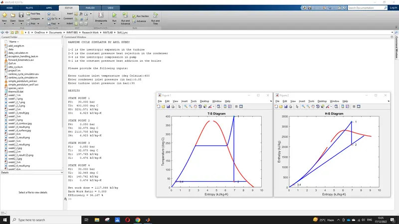
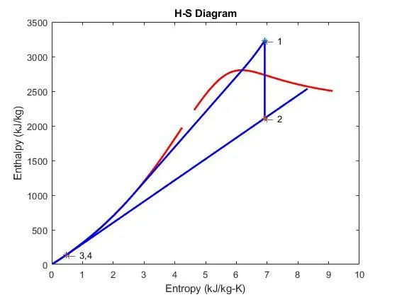
The above code produces the following output for Turbine inlet temperature = 400 deg C, Condenser Pressure = 0.05 bar and Turbine Inlet pressure = 30 bar:

RANKINE CYCLE SIMULATOR BY ANIL DUBEY

1-2 is the isentropic expansion in the turbine
2-3 is the constant pressure heat rejection in the condenser
3-4 is the isentropic compression in pump
4-1 is the constant pressure heat addition in the boiler

Please provide the following inputs:

Enter turbine inlet temperature (deg Celsius):400
Enter condenser inlet pressure (in bar):0.05
Enter turbine inlet pressure (in bar):30

RESULTS

STATE POINT 1
P1: 30.000 bar
T1: 400.000 deg C
H1: 3231.571 kJ/kg
S1: 6.923 kJ/kg-K

STATE POINT 2
P2: 0.050 bar
T2: 32.875 deg C
H2: 2110.708 kJ/kg
S2: 6.923 kJ/kg-K

STATE POINT 3
P3: 0.050 bar
T3: 32.875 deg C
H3: 137.765 kJ/kg
S3: 0.476 kJ/kg-K

STATE POINT 4
P4: 30.000 bar
T4: 32.945 deg C
H4: 140.762 kJ/kg
S4: 0.476 kJ/kg-K

Net work done = 1117.866 kJ/kg
Back Work Ratio = 0.003
Efficiency = 36.167 %

Figure 1 (T-S Diagram)

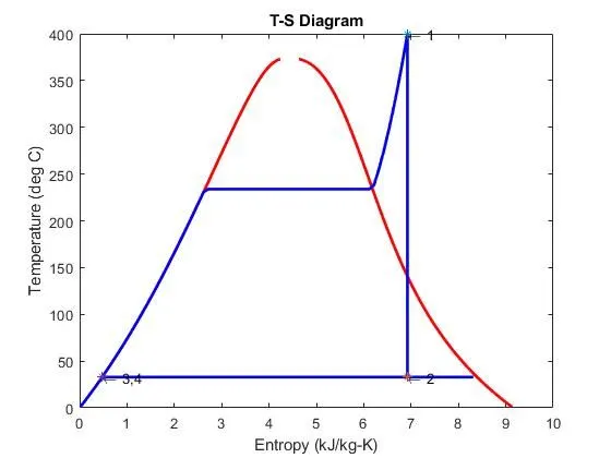
Figure 2 (H-S Diagram)

SCREENSHOT OF THE OUTPUT SCREEN WITH T-S AND H-S PLOTS: