Project 2 - Rankine cycle Simulator
Aim: Write a program in MATLAB to create a Rankine Cycle Simulator.
Objectives:
- Calculate State Points Variables of Rankine Cycle based on given user inputs.
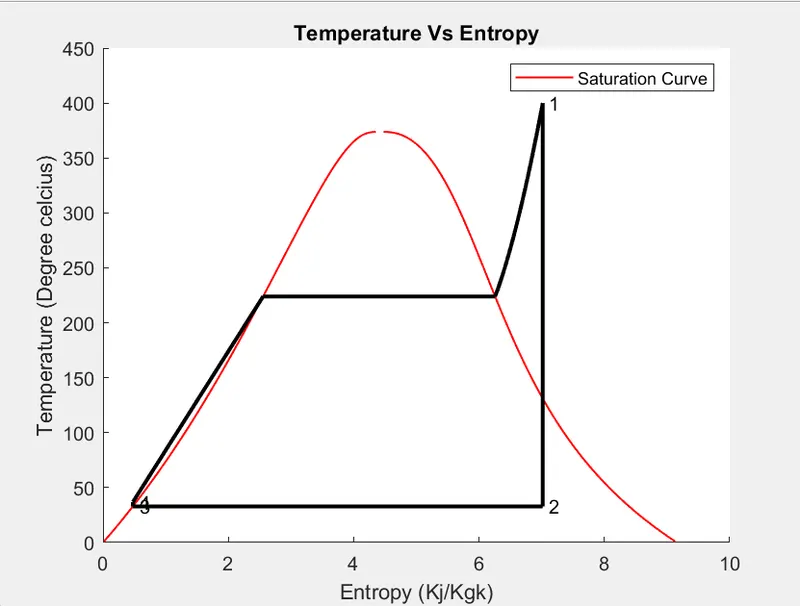
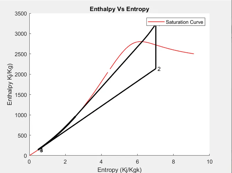
- Plot T-S, H-S for the given set of inputs and calculate Turbine work, work done on pump, Net work done, Thermal efficiency of the cycle.
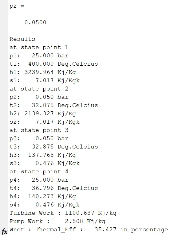
- Display results for all the state points variables in the Command window.
Solution:
Rankine Cycle:
It is a Thermodynamic cycle which describes working process of Steam turbine, Steam Engine and Heat Engine. It provides Useful work by extracting mechanical energy from the heat source. A pictorial representation Steam Turbine working on Rankine cycle process is given in below figure. 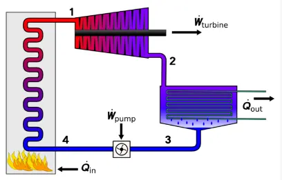
Working:
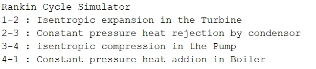
In steam turbine water is being fed to Boiler, where it gets boiled until it gets converted into high pressure steam by constant pressure heat addition process (Qin). Then, it supplied to Turbine, where steam gets expand and heat energy is converted into mechanical energy(Wt) which basically uses to generate an electricity with the help of Generator. Then, expanded steam is supplied to Condenser where it gets converted back to water by constant pressure heat rejection process(Qout). This water is sent to Pump in order to increase pressure for boiler input by Wp.
Equations:
Qin = h1 – h4
Wt = h1 – h2
Qout = h2- h3
Wp = h4 – h3
Wnet = Wt – Wp
Thermal Efficiency = (Wnet/Qin) *100
Inputs:
Turbine Inlet Pressure, p1 = 30 bar
Turbine Inlet Temperature, t1 = 400° C
Turbine Outlet Pressure, p2 = 0.05 bar = Condenser Inlet Pressure, p3
MATLAB Program:
% Rankin_cycle_simulator
clear all
close all
clc

% Printing Processes

fprintf('Rankin Cycle Simulator\n');
fprintf('1-2 : Isentropic expansion in the Turbine\n');
fprintf('2-3 : Constant pressure heat rejection by condensor\n');
fprintf('3-4 : isentropic compression in the Pump\n');
fprintf('4-1 : Constant pressure heat addion in Boiler\n');

% Inputs
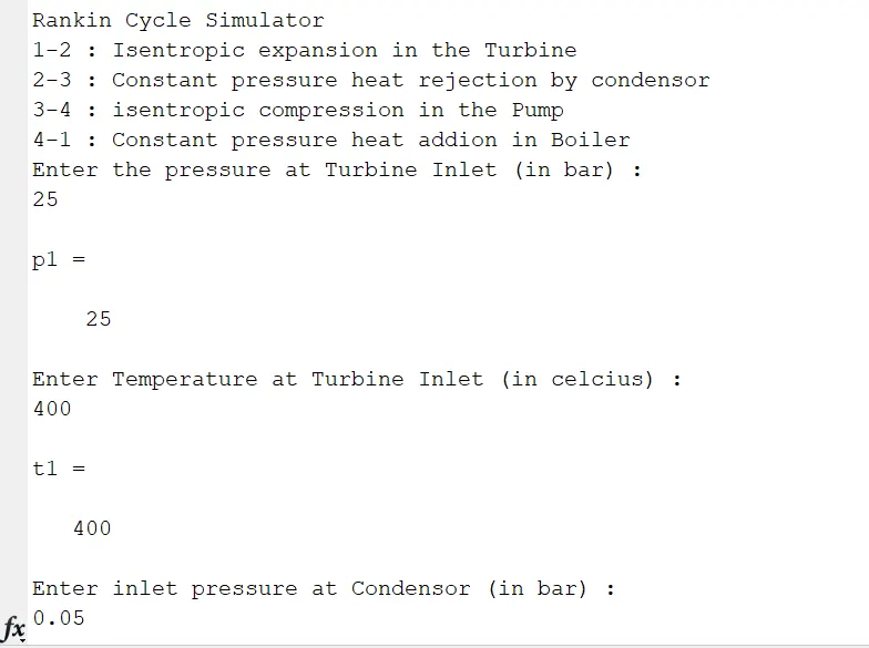
p1 = input('Enter the pressure at Turbine Inlet (in bar) :\n')
t1 = input('Enter Temperature at Turbine Inlet (in celcius) :\n')
p2 = input('Enter inlet pressure at Condensor (in bar) :\n')

% p1 = 25
% t1 = 400
% p2=0.05

%Calculating State Ponit Variables
%State point 1
h1 = XSteam('h_pT',p1,t1);
s1 = XSteam('s_pT',p1,t1);

%State point 2
s2 = s1 ;
sf2 = XSteam('sL_p',p2);
sg2 = XSteam('sV_p',p2);

x2 = (s2-sf2)/(sg2-sf2);

hf2 = XSteam('hL_p',p2);
hg2 = XSteam('hV_p',p2);
h2 = hf2 + (x2*(hg2-hf2));

%State Point 3
p3 = p2;
s3 = XSteam('sL_p',p3);
h3 = XSteam('hL_p',p3);

%State point 4
p4 = p1;
s4 = s3;

%Workdone by Turbine
Wt = h1 - h2;

%workdone on Pump
v3 = XSteam('vL_p',p3);
Wp = v3*(p4-p3)*100;
h4 = h3+Wp;

%Net workdone
Wnet = Wt - Wp;

%Heat addition to Boiler
Qin = h1 - h4;

%Heat rejection to atm from Condensor
Qout = h2 - h3;

%Thermal efficiency
Thermal_eff = (Wnet/Qin)*100;

%Calculating Temperatures at State points 2,3,4
t3 = XSteam('Tsat_p',p3);
t2 = t3;

cp4 = XSteam('cp_ps',p4,s4);
cv4 = XSteam('cv_ps',p4,s4);

k = cp4/cv4;

t4 = t3/(p3/p4)^((k-1)/k);

%Calculating T, H, S for required points

t6 = XSteam('Tsat_p',p1);
s5 = XSteam('sL_p',p1);
s6 = XSteam('sV_p',p1);
h5 = XSteam('hL_p',p1);
h6 = XSteam('hV_p',p1);
t5 = t6;

%plotting Saturation Curve

T = linspace(1,375,1000);
for i = 1 : length(T)
    sf(i) = XSteam('sL_T',T(i));
    sg(i) = XSteam('sV_T',T(i));
    hf(i) = XSteam('hL_T',T(i));
    hg(i) = XSteam('hV_T',T(i));
end

%Plotting T-S diagram
figure(1)
hold on
plot(sf,T,'Color','r','LineWidth',1)
plot(sg,T,'Color','r','LineWidth',1)
plot([s1 s2],[t1 t2],'k','LineWidth',2)
plot([s2 s3],[t2 t3],'k','LineWidth',2)
plot([s3 s4],[t3 t4],'k','LineWidth',2)
plot([s4 s5],[t4 t5],'k','LineWidth',2)
plot([s5 s6],[t5 t6],'k','LineWidth',2)

sc1 = linspace(s6,s1,1000);
for l = 1:length(sc1)
    Tc1(l) = XSteam('T_ps',p1,sc1(l));
end

plot(sc1,Tc1,'k','LineWidth',2)

text(s1+0.1,t1,'1')
text(s2+0.1,t2,'2')
text(s3+0.1,t3,'3')
text(s4+0.1,t4,'4')
title('Temperature Vs Entropy')
xlabel('Entropy (Kj/Kgk)')
ylabel('Temperature (Degree celcius)')
legend('Saturation Curve')

%Plotting H-S diagram
figure(2)
hold on
plot(sf,hf,'r','LineWidth',1)
plot(sg,hg,'r','LineWidth',1)
plot([s1 s2],[h1 h2],'k','LineWidth',2)
plot([s2 s3],[h2 h3],'k','LineWidth',2)
plot([s3 s4],[h3 h4],'k','LineWidth',2)

hc = linspace(h4,h5,100);
for k = 1 : length(hc)
    sch(k) = XSteam('s_ph',p1,hc(k));
end

plot(sch,hc,'k','LineWidth',3)25
plot([s5 s6],[h5 h6],'k','LineWidth',2)

for m = 1:length(sc1)
    hc1(m) = XSteam('h_ps',p1,sc1(m));
end

plot(sc1,hc1,'k','LineWidth',2)

text(s1+0.1,h1,'1')
text(s2+0.1,h2,'2')
text(s3+0.1,h3,'3')
text(s4+0.1,h4,'4')
title('Enthalpy Vs Entropy')
xlabel('Entropy (Kj/Kgk)')
ylabel('Enthalpy Kj/Kg)')
legend('Saturation Curve')

%Displaying results
disp('Results')

fprintf('at state point 1\n')
fprintf('p1: %8.3f bar\n',p1);
fprintf('t1: %8.3f Deg.Celcius\n',t1)
fprintf('h1: %8.3f Kj/Kg\n',h1)
fprintf('s1: %8.3f Kj/Kgk\n',s1)

fprintf('at state point 2\n')
fprintf('p2: %8.3f bar\n',p2);
fprintf('t2: %8.3f Deg.Celcius\n',t2)
fprintf('h2: %8.3f Kj/Kg\n',h2)
fprintf('s2: %8.3f Kj/Kgk\n',s2)

fprintf('at state point 3\n')
fprintf('p3: %8.3f bar\n',p3);
fprintf('t3: %8.3f Deg.Celcius\n',t3)
fprintf('h3: %8.3f Kj/Kg\n',h3)
fprintf('s3: %8.3f Kj/Kgk\n',s3)

fprintf('at state point 4\n')
fprintf('p4: %8.3f bar\n',p4);
fprintf('t4: %8.3f Deg.Celcius\n',t4)
fprintf('h4: %8.3f Kj/Kg\n',h4)
fprintf('s4: %8.3f Kj/Kgk\n',s4)

fprintf('Turbine Work : %8.3f Kj/kg\n',Wt)
fprintf('Pump Work : %8.3f Kj/kg\n',Wp)
fprintf('Wnet : %8.3 Kj/kg\n',Wnet)
fprintf('Thermal_Eff : %8.3f in percentage\n',Thermal_eff)
Plots :
T-S diagram
H-S diagram:
Output:
Conclusion:
A Rankine Cycle Simulator has been created and T-S, H-S as well as required output was obtained from the program with given set of inputs.
References: