Project 2 - Rankine cycle Simulator
Rankine cycle: The ideal cycle for the vapour power cycle
Many of the impracticalities associated with the Carnot cycle can be eliminated by superheating the steam in the boiler and condensing it completely in the condenser, as shown schematically on a T-s diagram. The cycle that results is the Rankine cycle, which is the ideal cycle for vapor power plants.
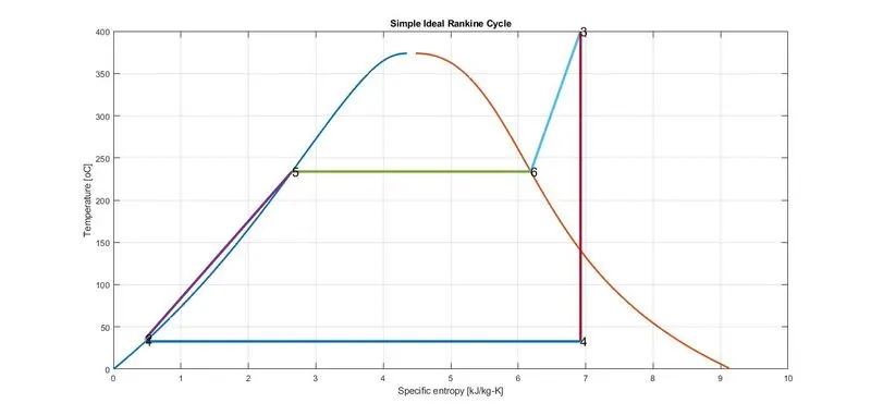
The ideal Rankine cycle does not involve any internal irreversibilities and consists of the following four processes:
1-2 Isentropic compression in a pump
2-3 Constant pressure heat addition in a boiler
3-4 Isentropic expansion in a turbine
4-1 Constant pressure heat rejection in a condenser
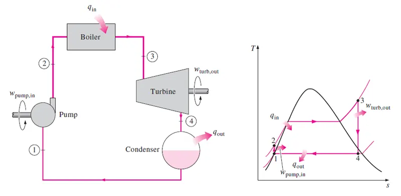
Figure: Simple Ideal Rankine Cycle
Energy Analysis of the Ideal Rankine Cycle
All four components associated with the Rankine cycle (the pump, boiler, turbine, and condenser) are steady-flow devices, and thus all four processes that make up the Rankine cycle can be analyzed as steady-flow processes.
Steady flow energy equation per unit mass:
`h_i+c_i^2/2+gz_i+q=h_o +c_o^2/2+gz_o + w_(cv)`
Here, `i` stands for inlet and `o` stands for the outlet
`h` = specific enthalpy (kJ/kg)
`c^2/2` = Kinetic energy (kJ/kg)
`gz` = Potential energy (kJ/kg)
`q` = Heat transfer (kJ/kg)
`w_(cv)` = Control volume work transfer (kJ/kg)
The kinetic and potential energy changes of the steam are usually small relative to the work and heat transfer terms and are therefore usually neglected. so steady flow energy equation becomes.
`h_i+q=h_o + w_(cv)`
Now apply the steady flow energy equation to each component.
Pump
`h_1+q=h_2 + w_(cv)`
`h_1+0=h_2 + w_(pump)`
`w_(pump)=h_1-h_2=-int_1^2vdP=-v_1(P_2-P_1) =-100v_1(P_2-P_1)`kJ/kg
Boiler
`h_2+q=h_3 + w_(cv)`
`h_2+q_i=h_3 + 0`
`q_i=h_3-h_2` kJ/kg
Turbine
`h_3+q=h_4 + w_(cv)`
`h_3+0=h_4 + w_(turb)`
`w_(turb)=h_3-h_4` kJ/kg
Condenser
`h_4+q=h_1 + w_(cv)`
`h_4+q_(out)=h_1 + 0`
`q_(out)=h_1-h_4` kJ/kg
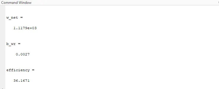
Net work output, `W_(Net)=w_(turb)-w_(pump)=q_i-q_(out)`
Back work ratio, `b_(wr)=w_(pump)/w_(turb)`
Given data:
Turbine inlet temperature `T_3=400^oC`
Turbine inlet pressure `P_3=P_2=30` bars
Turbine outlet pressure = Condenser inlet pressure `P_4=P_1=0.05` bars
MATLAB Code
%% Simple Ideal Rankine Cycle
clc
clear all
close all

%% Given data
T3=400;                      % turbine inlet temperature in degree celcius
p3=30;                       % turbine inlet pressure in bar
p4=0.05;                     % turbine outlet pressure

%% computation of pump work
v=XSteam('vL_p',p4);         % specific volume of saturated water at 0.05 bar pressure
p2=p3;                       % since boiler operates at constant pressure
p1=p4;                       % since condenser operates at constant pressure
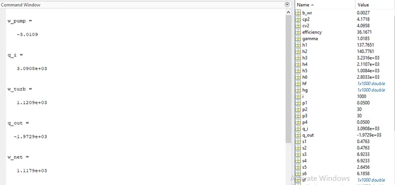
w_pump=-100*v*(p2-p1);       % work unit is in kJ/kg

%% Computation of heat input to boiler
h3=XSteam('h_pT',p3,T3);    % enthalpy of superheated steam at 30 bar and 400 degC
h1=XSteam('hL_p',p1);       % enthalpy of saturated waterat 0.05 bar
h2=h1-w_pump;               % enthalpy of subcooled water
q_i=h3-h2;                  % heat input to boiler at 30 bar pressure

%% computation of turbine work
s3=XSteam('s_pT',p3,T3);    % entropy of superheated steam at 30 bar and 400 degC
s4=s3;                      % isentropic process(reversible adiabatic)
h4=XSteam('h_ps',p4,s4);    % enthalpy of mixture
w_turb=h3-h4;               % turbine work

%% computation of heat rejection from condenser
q_out=h1-h4;

%% Net work output
w_net=w_turb-abs(w_pump);

%% Back work ratio
b_wr=abs(w_pump)/w_turb;

%% Thermal efficiency of Rankine cycle
efficiency=(w_net/q_i)*100;

%% calculation at state points 1,2,3,4,5 and 6
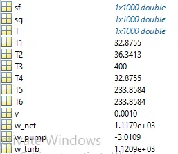
T1=XSteam('Tsat_p',p1);     % saturation temperature of water at 0.05 bar
s1=XSteam('sL_p',p1);       % specific entropy of saturated water at 0.05 bar
s2=s1;                      % isentropic process
cp2=XSteam('Cp_ps',p2,s2);  % specific isobaric heat capacity at 30 bar and s2 entropy
cv2=XSteam('Cv_ps',p2,s2);  % pecific isochoric heat capacity at 30 bar and s2 entropy
gamma=cp2/cv2;              % ratio of specific heat capacity
T2=T1*(p2/p1)^(gamma-1)/gamma;
T3=400;                     % superheated steam temperature at turbine inlet
T4=T1;                      % constant temperature heat rejection
T5=XSteam('Tsat_p',p3);     % saturation temperature corresponding to 30 bar
T6=T5;
s5=XSteam('sL_p',p3);       % saturated liquid entropy corresponding to 30 bar
s6=XSteam('sV_p',p3);       % saturated vapour entropy corresponding to 30 bar
h5=XSteam('hL_p',p3);       % saturated liquid enthalpy corresponding to 30 bar
h6=XSteam('hV_p',p3);       % saturated vapour enthalpy corresponding to 30 bar

%% saturation curve
T=linspace(1,375,1000);
for  i=1:length(T)
    sf(i)=XSteam('sL_T',T(i));
    sg(i)=XSteam('sV_T',T(i));
    hf(i)=XSteam('hL_T',T(i));
    hg(i)=XSteam('hV_T',T(i));
end

%% T-s diagram of Rankine cycle
figure(1)
plot(sf,T,'linewidth',2)                % saturated liquid curve
hold on
plot(sg,T,'linewidth',2)                % saturated vapour curve
plot([s1 s2],[T1 T2],'linewidth',3)     % pumping process
plot([s2 s5],[T2 T5],'linewidth',3)     % Process in Economiser
plot([s5 s6],[T5 T6],'linewidth',3)     % Process in Boiler
plot([s6 s3],[T6 T3],'linewidth',3)     % Process in Superheater
plot([s3 s4],[T3 T4],'linewidth',3)     % Process in Turbine
plot([s4 s1],[T4 T1],'linewidth',3)     % Process in Condenser
xlabel('Specific entropy [kJ/kg-K]')
ylabel('Temperature [oC]')
title('Simple Ideal Rankine Cycle')
grid on
text(s1,T1,'1','FontSize',15)
text(s2,T2,'2','FontSize',15)
text(s5,T5,'5','FontSize',15)
text(s6,T6,'6','FontSize',15)
text(s3,T3,'3','FontSize',15)
text(s4,T4,'4','FontSize',15)

%% h-s diagram of Rankine cycle
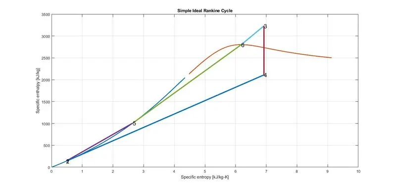
figure(2)
plot(sf,hf,'linewidth',2)               % saturated liquid curve
hold on
plot(sg,hg,'linewidth',2)               % saturated vapour curve
plot([s1 s2],[h1 h2],'linewidth',3)     % pumping process
plot([s2 s5],[h2 h5],'linewidth',3)     % Process in Economiser
plot([s5 s6],[h5 h6],'linewidth',3)     % Process in Boiler
plot([s6 s3],[h6 h3],'linewidth',3)     % Process in Superheater
plot([s3 s4],[h3 h4],'linewidth',3)     % Process in Turbine
plot([s4 s1],[h4 h1],'linewidth',3)     % Process in Condenser
xlabel('Specific entropy [kJ/kg-K]')
ylabel('Specific enthalpy [kJ/kg]')
title('Simple Ideal Rankine Cycle')
grid on
text(s1,h1,'1','FontSize',15)
text(s2,h2,'2','FontSize',15)
text(s5,h5,'5','FontSize',15)
text(s6,h6,'6','FontSize',15)
text(s3,h3,'3','FontSize',15)
text(s4,h4,'4','FontSize',15)