Project 2 - Rankine cycle Simulator
clear all
close all
clc

% display
disp('RANKINE CYCLE SIMULATION');
disp('1-2 isentropic expansion in turbine');
disp('2-3 constant pressure heat rejection from condenser');
disp('3-4 isentropic compression in pump');
disp('4-1 constant pressure heat addition from boiler');

% Inputs
t_1= input('enter the temperature at turbine inlet (in °C):');
p_1= input('enter the pressure at turbine inlet (in bar):');
p_2= input('enter the pressure at turbine outlet (in bar):');

% Assuming t_1= 400°C, p_1= 30bar, p_2= 0.05 bar
% state points at 1
p1=p_1;
t1=t_1;
%s1= XSteam('s_pT',p1,t1)
s1= XSteam('s_pT',p1,t1);
h1= XSteam('h_pT',p1,t1);
ts1= XSteam('Tsat_p', p1);
sf1= XSteam('sL_p', p1);
sg1= XSteam ('sV_p',p1);
hf1= XSteam('hL_p',p1);
hg1= XSteam('hV_p',p1);

% state points at 2
s2=s1;
p2=p_2;
t2= XSteam('Tsat_p',p2);
ts2= XSteam('Tsat_p',p2);
sf2= XSteam('sL_p', p2);
sg2= XSteam ('sV_p',p2);
hf2= XSteam('hL_p',p2);
hg2= XSteam('hV_p',p2);
x2= ((s2-sf2)/(sg2-sf2));
h2= hf2+(x2*(hg2-hf2));

% state points at 3
p3=p2;
t3=t2;
s3= XSteam('sL_p',p3);
v3= XSteam('vL_p',p3);

sf3= XSteam('sV_p', p3);
sg3= XSteam ('sL_p',p3);
hf3= XSteam('hV_p',p3);
hg3= XSteam('hL_p',p3);
x3= ((s3-sf3)/(sg3-sf3));
h3= hf3+(x3*(hg3-hf3));

% Calculation of 'g' using gamma
cp4= XSteam('cpL_p',p3);
cv4= XSteam('cvL_p',p3);
gamma= (cp4/cv4);
g= (gamma-1)/gamma;

% State points at 4
p4=p1;
s4=s3;
h4= XSteam('h_ps',p4,s4);
t4= t3*((p4/p3)^g);

% Work done calculation and thermal efficiency
wt= h1-h2;
wp= h4+h3;
wnet= wt-wp;
Qin= h1-h4;
Qout= h2-h3;
Ntherm= (wnet/Qin)*100;
s.s.c= 3600/wt;

temp= linspace(1,400,500);
for i= 1:length(temp)
        a(i)= XSteam('hL_T', temp(i));
        b(i)= XSteam('hV_T', temp(i));
        c(i)= XSteam('sL_T', temp(i));
        d(i)= XSteam('sV_T', temp(i));
end

% Plot 1
figure (1)
hold on
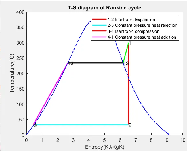
plot([s1 s2],[t1 t2],'color','r','linewidth',2)
text(s1,t1,'1');
text(s2,t2,'2');
plot([s2 s3],[t2 t3],'color','c','linewidth',2)
text(s3,t3,'3');
plot([s3 s4],[t3 t4],'color','r','linewidth',2)
text(s4,t4,'4');
plot([s4 sf1],[t4 ts1], 'color','m','linewidth',2)
text(sf1,ts1,'4S');
plot([sf1 sg1],[ts1 ts1],'color','k','linewidth',2)
text(sg1,ts1,'1S')
plot([sg1 s1],[ts1 t1],'color','g','linewidth',2)
plot(c,temp,'color','b','linestyle','-.','linewidth',1.5)
plot(d,temp,'color','b','linestyle','-.','linewidth',1.5)
title('T-S diagram of Rankine cycle')
xlabel('Entropy(KJ/KgK)')
ylabel('Temperature(°C)')
legend('1-2 Isentropic Expansion','2-3 Constant pressure heat rejection','3-4 Isentropic compression','4-1 Constant pressure heat addition')

% Plot2
figure(2)
hold on
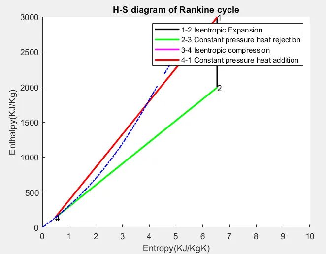
plot([s1 s2],[h1 h2],'color','k','linewidth',2)
text(s1,h1,'1');
plot([s2 s3],[h2 h3],'color','g','linewidth',2)
text(s2,h2,'2');
plot([s3 s4],[h3 h4],'color','m','linewidth',2)
text(s3,h3,'3');
plot([s4 s1],[h4 h1],'color','r','linewidth',2)
text(s4,h4,'4');
plot(c,a,'color','b','linestyle','-.','linewidth',1.5)
plot(d,b,'color','b','linestyle','-.','linewidth',1.5)
title('H-S diagram of Rankine cycle')
xlabel('Entropy(KJ/KgK)')
ylabel('Enthalpy(KJ/Kg)')
legend('1-2 Isentropic Expansion','2-3 Constant pressure heat rejection','3-4 Isentropic compression','4-1 Constant pressure heat addition')

% Displaying all the values at states 1-4
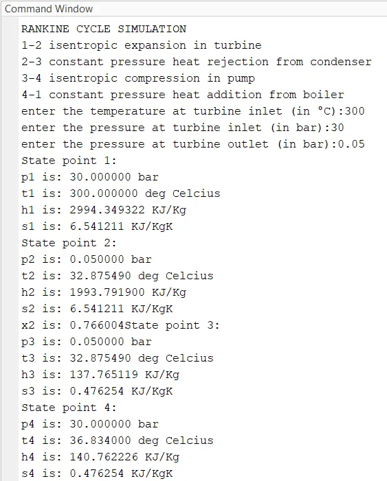
disp('State point 1:')
fprintf('p1 is: %f bar\n', p1)
fprintf('t1 is: %f deg Celcius\n', t1)
fprintf('h1 is: %f KJ/Kg\n', h1)
fprintf('s1 is: %f KJ/KgK\n', s1)

disp('State point 2:')
fprintf('p2 is: %f bar\n', p2)
fprintf('t2 is: %f deg Celcius\n', t2)
fprintf('h2 is: %f KJ/Kg\n', h2)
fprintf('s2 is: %f KJ/KgK\n', s2)
fprintf('x2 is: %f', x2)

disp('State point 3:')
fprintf('p3 is: %f bar\n', p3)
fprintf('t3 is: %f deg Celcius\n', t3)
fprintf('h3 is: %f KJ/Kg\n', h3)
fprintf('s3 is: %f KJ/KgK\n', s3)

disp('State point 4:')
fprintf('p4 is: %f bar\n', p4)
fprintf('t4 is: %f deg Celcius\n', t4)
fprintf('h4 is: %f KJ/Kg\n', h4)
fprintf('s4 is: %f KJ/KgK\n', s4)

% displaying thermal efficiency, work done
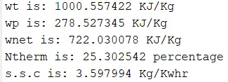
fprintf('wt is: %f KJ/Kg\n', wt)
fprintf('wp is: %f KJ/Kg\n', wp)
fprintf('wnet is: %f KJ/Kg\n', wnet)
fprintf('Ntherm is: %f percentage\n', Ntherm)
fprintf('s.s.c is: %f Kg/Kwhr\n', s.s.c)
Explanation for the code:
Generally to clear the workspace history, commands and to close all the commands clear all, close all and clc is used. The program is used here is to simulate the working of rankine cycle and to generate the varoius plots between temperature Vs Enthalpy & temperature Vs Entropy. As we know, there are 4 process involved in rankine cycle, 1-2 isentropic expansion, 2-3 constant pressure haet rejection, 3-4 isentropic compression and 4-1 constant pressure heat addition. Using display command, we are going to display the process names and the name of the cycle in the command window. Assuming, turbine inlet temperature t_1= 400 °C, turbine inlet pressure p_1= 30 bar and turbine outlet pressure p_2= 0.05 bar. During the state 1, by declaring t1 as t_1, p1 as p_1, the values of t_1 and p_1 are assigned to t1 and p1 respectively. Taking the p1 & t1 values in steam table, XSteam value is taken. Using XSteam value, s1, h1, ts1, sf1, sg1, hf1, hg1 are calculated. In state 2, during constant pressure and isentropic process, s1=s2 and turbine output pressure, p2=p_2=0.05 bar is assumed. Then t2, ts2, sf2, sg2, hf2, hg2, x2, h2 are calculated. At state point 3, there is isentropic compression process in which p3=p2, t3=t2 and using those values v3, s3, sf3, sg3, hf3, hg3, x3, h3 are calculated. Using cp4, cv4 gamma is calculated. Then using gamma, g is calculated. At state point 4, at constant pressure heat rejection process p1=p4, s3=s4 then h4 and t4 are calculated. Now we can find all the thermodynamic parameters from stae points 1-4. Now work done at turbine and pumps are calculated. To calculate net work done, we can find the difference between work done by the turbine and work done by the pump. Then we should calculate Qin, Qout, Specific heat consumption (S.S.C) and thermal efficiency is calculated. Then using plot command, we are plotting graphs between temperature vs enthalpy, temperature vs entropy. Finally, using printf command we are displaying the thermodynamic parameters of all four state points in command window.
Output:
T-S diagram for Rankine cycle
H-S diagram for Rankine cycle
Calculation of Work done and thermal efficiency:
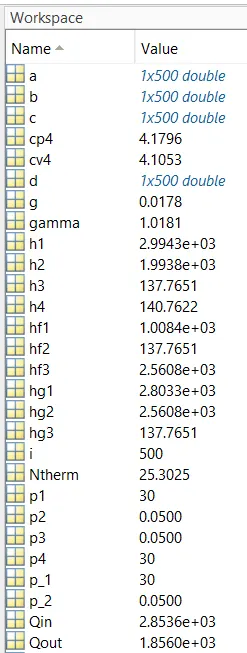
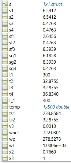
Workspace:
Errors faced while programming:
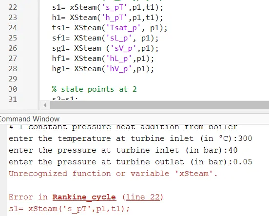
From the Xsteam data table, in the variable XSteam , 'X' and 'S' should in upper cases. If it is not as per the table it will say "invalid identifier".
Conclusion: Thus, we have successfully simulated the rankine cycle using matlab and plotted graphs between temperature Vs Enthalpy and Temperature Vs Entropy.
Reference: