Project 2 - Rankine cycle Simulator

RANKINE CYCLE SIMULATOR

Understand the concept of Rankine cycle by referring to the standard thermal engineering textbook.

Create a Rankine cycle simulator using OCTIVE/MATLAB.

Required inputs:

• Turbine inlet temperature = 400
• Turbine inlet pressure = 30 bars
• Turbine outlet pressure = 0.05 bars = condenser inlet pressure

Calculating the following output:

• Network output
• Back work ratio

Definitions:

• Working fluid is alternately vaporized and condensed as it recirculates in the closer cycle
• Water is typically used as the working fluid because of its low cost and relatively large value enthalpy of vaporization.
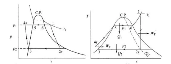
• The standard vapor cycle that excludes internal irreversibility’s is called the ideal Rankine cycle

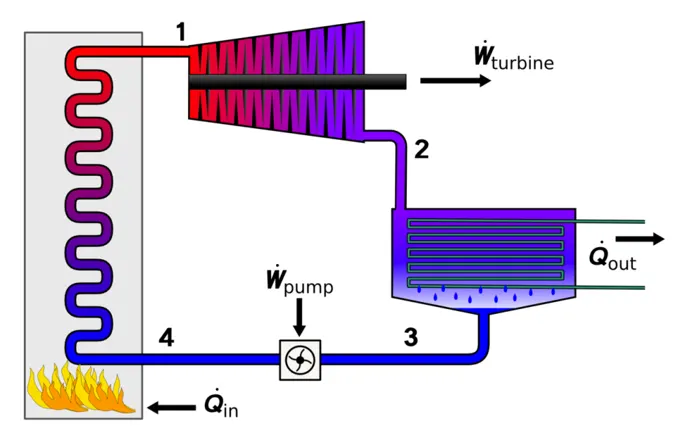
In the above figure

• The condensation process is allowed to proceed to completion between state points 4 to 1

-provides a saturated liquid at 1

• The water at state point 1 can be conveniently pumped to the boiler pressure at state point 2
• but water is not at the saturation temperature corresponding to the boiler pressure
• heat must be added to change the water at 2 to saturated water at ‘a’
• when heat is added at non-constant temperature (between 2-a),the cycle efficiency will be decrease

Four components of the Rankine cycle:

1. Pump
2. Boiler
3. Turbine
4. Condenser

Four processes of the Rankine cycle:

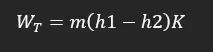
1-2: Isentropic Expansion

Turbine (1-2): superheated steam enters into the turbine and expands isentropically resulting in the production of work. The shaft of the turbine is connected to the generator. This results in the production electricity i.e. mechanical energy gets converted into electrical energy. Work product by the turbine,

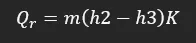
2-3: constant pressure heat rejection

Condenser (2-3): he expanded vapor is then passed through a condenser, where it gets condensed and converts into liquid again. This liquid is again pumped to the boiler.

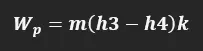
3-4: Isentropic compression by the pump

Condenser (3-4): The water enters into the pump in a saturated state. Then the liquid is compressed and converts into liquid again pumped to the boiler.

4-1: constant pressure heat addition

Boiler (4-1): the water enters into the boiler as compressed and leaves as superheated from the boiler. Thus, the phase change from liquid to vapor. The heat supplied by the boiler is

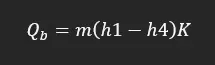
Hear we take mass flow rate m = 1 for this code.

MATLAB coding details:

clear all
close all
clc

disp('RANKINE CYCLE SIMULATOR')
disp('1-2 Isentropic Expansion in the Turbine')
disp('2-3 Constant Pressure Heat Rejection by the Condenser')
disp('3-2 Isentropic Compression in the Pump')
disp('4-1 Constant pressure Heat Addition by the Boiler')

%Required Inputs
P1 = input('. Turbine Inlet Pressure (in bar):');
T1 = input('. Turbine Inlet Temperature (in Degree celsius):');
P2 = input('. Turbine Outlet Pressure (in bar):');

disp('RESULTS')

%getting Cp and Cv values from Xsteam
%Cp and Cv assumed and will not change with temperature

%Input detail for Vapour
high_CpV = XSteam('CpV_p',P1);
low_CpV = XSteam('CpV_p',P2);
high_CvV = XSteam('CvV_p',P1);
low_CvV = XSteam('CvV_p',P2);

%Input detail for Liquid
high_CpL = XSteam('CpL_p',P1);
low_CpL = XSteam('CpL_p',P2);
high_CvL = XSteam('CvL_p',P1);
low_CvL = XSteam('CvL_p',P2);

%Redading from Xsteam file for important parameters

%Input detail for Pressure
T1s = XSteam('Tsat_p',P1);
S1g = XSteam('sV_p',P1);
S1f = XSteam('SL_p',P1);
S1fg = S1g - S1f;
H1f = XSteam('hL_p',P1);
H1g = XSteam('hV_p',P1);
H1fg = H1g - H1f;

%Input detail for Low Pressure
T2s = XSteam('Tsat_p',P2);
S2g = XSteam('sV_p',P2);
S2f = XSteam('SL_p',P2);
S2fg = S2g - S2f;
H2f = XSteam('hL_p',P2);
H2g = XSteam('hV_p',P2);
H2fg = H2g - H2f;

%State point 1
disp('At state point 1:')
fprintf('P1 is : %f Barn',P1)

fprintf('T1 is :%f Deg celsiusn',T1)
H1 = XSteam('h_pt',P1,T1);

fprintf('H1 is :%f kJ/kgn',H1)
S1 = XSteam('S_pt',P1,T1);

fprintf('S1 is :%f kJ/kgknn',S1)

%state point 2
disp('At state point 2:')
fprintf('P2 is :%f Barn',P2)
S2 = S1;
fprintf('S2 is :%f kJ/kgkn',S2)

%Dryness Fraction of point 2 in T-s
if (S2<=S2g)
X2 = (S2 - S2f)/(S2fg);
else
x2 = 1;
end

fprintf('X2 is :%f n',X2)

%Calculating T2 for superheat, dry, wet
if (X2<1)
T2 = T2s;
else
end
%now calculating T2 by s2=s2g+low_cpV*(log(T2/T2s))

T2 = (T2s+273.15)*exp((S2-S2g)/low_CpV);
T2=T2-273.15;
fprintf('T2 is :%f Deg celsius n',T2)
if (X2<1)
H2 = H2f + X2* H2fg;
else
H2=h2g+low_CpV*(T2-T2s);
end
fprintf('H2 is :%fkJ/kgn',H2)

%State point 3 where assuming no subcolling
disp('At state point 3:')
P3 = P2;
fprintf('P3 is :%f Barn',P3)
V3 = XSteam('vL_p',P3);

T3 = T2s;
fprintf('T3 is :%f Deg celsiusn',T3)
H3 = H2f;
fprintf('H3 is :%f kJ/kgn',H3)
S3 = S2f;
fprintf('S3 is :%f kJ/kJknn',S3)

%State point 4
disp('At state point 4:')
P4 = P1;
fprintf('P4 is :%f Barn',P4)
S4 = S3;
fprintf('S4 is :%f kJ/kgkn',S4)
Wp = V3*(P4-P3)*100;
H4 = Wp + H3
fprintf('H4 is :%f kJ/kgn',H4)

%For calculating T4 s4=s3=sf1-high_cpL*ln(tis/t4)
term = exp((S1f-S4)/high_CpL);
T4=T1s/term;
fprintf('T4 is :5f deg celsius nn',T4)

%Work done, heat, SSC and efficiency calculations
Wt = H1 - H2;
fprintf('Work by turbine is :%f kJ/kgn',Wt)
fprintf('Work by compressor is :%f kJ/kgn',Wp)

Wnet = Wt - Wp;
fprintf('Net work done is :%f kJ/kgn',Wnet)

Qin = H1 - H4;
eff_thermal = Wnet/Qin; %Efficiency

fprintf('thermal efficiency is :%f',eff_thermal);disp('%')
SSC = 3600 / Wt;

fprintf('S.S.C is :%f kg/kWh',SSC)

%Calculation for plotting Liquid and Vapour lines

temp = linspace(1,373,500);
for i = 1:length(temp)
H_L(i) = XSteam('hL_T',temp(i));
H_V(i) = XSteam('hV_T',temp(i));
S_L(i) = XSteam('sL_T',temp(i));
S_V(i) = XSteam('sV_T',temp(i));
end

%ploting T-S and H-S diagrams

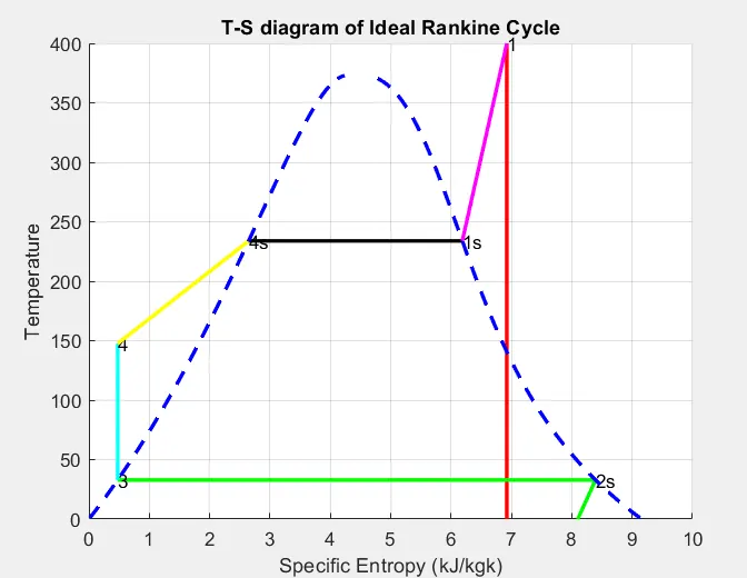
%T-s diagram of Ideal Rankine Cycle

figure(1)
title('T-S diagram of Ideal Rankine Cycle')
xlabel('Specific Entropy (kJ/kgk)')
ylabel('Temperature')
grid on
hold on
plot([S1 S2],[T1 T2],'r','linewidth',2)
text(S1,T1,'1')

text(S2,T2,'2')
plot([S2 S2g],[T2 T2s],'g','linewidth',2)
text(S2g,T2s,'2s')
plot([S2g S3],[T2s T3],'g','linewidth',2)

text(S3,T3,'3')
plot([S3 S4],[T3 T4],'c','linewidth',2)

text(S4,T4,'4')
plot([S4 S1f],[T4 T1s],'y','linewidth',2)
text(S1f,T1s,'4s')

plot([S1f S1g],[T1s T1s],'k','linewidth',2)
text(S1g,T1s,'1s')
plot([S1g S1],[T1s T1],'m','linewidth',2)


plot(S_L, temp, 'b','linestyle','--', 'linewidth',2)
plot(S_V, temp, 'b','linestyle','--', 'linewidth',2)

xlim([0.00 10.00])
ylim([0 400])

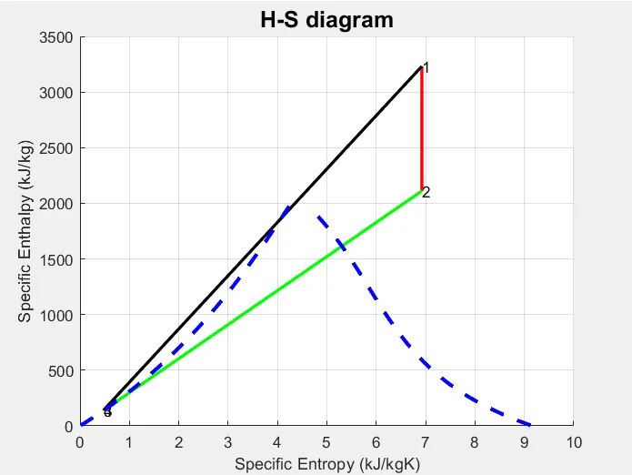
%H-S Diagram

figure(2)
title('H-S diagram','FontSize',15)
ylabel('Specific Enthalpy (kJ/kg)')
xlabel('Specific Entropy (kJ/kgK)')
grid on

hold on
plot([S1 S2],[H1 H2],'r','linewidth',2)
text(S1,H1,'1')

plot([S2 S3],[H2 H3],'g','linewidth',2)
text(S2,H2,'2')

plot([S3 S4],[H3 H4],'r','linewidth',2)
text(S3,H3,'3')

plot([S4 S1],[H4 H1],'k','linewidth',2)
text(S4,H4,'4')

plot(S_L, H_L, 'b','linestyle','--', 'linewidth',2.5)
plot(S_V, H_L, 'b','linestyle','--', 'linewidth',2.5)

xlim([0.00 10.00])
ylim([0 3500])

Code Explanation:

1. Display some information about Rankine cycle.
2. Take the inputs from user.
3. Find the state point properties (temperature, enthalpy, entropy) from the Xsteam.m file.
4. Calculate the turbine work, pump work, network, thermal efficiency, specific fuel consumption.
5. Plot the saturation dome along with the Rankine cycle process curves in T-S diagram.
6. Plot the saturation dome along with the Rankine cycle process curves in H-S diagram.
7. Print the output variables.

Output results:

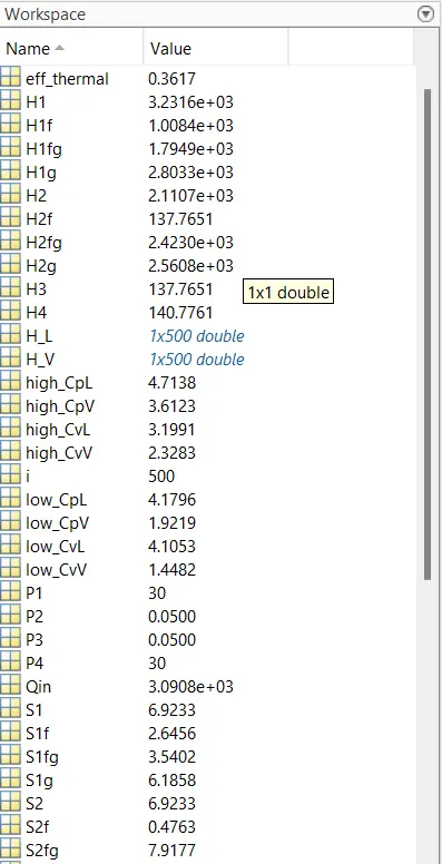
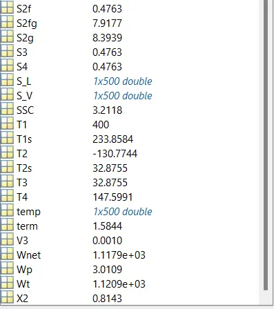
This result depends upon the input of

• Turbine inlet temperature = 400
• Turbine inlet pressure = 30 bars
• Turbine outlet pressure = 0.05 bars = condenser inlet pressure

Workspace:

RANLINE CYCLE: IDEAL CYCLE FOE VAPOUR POWER CYCLE

Process 1-2: Reversible adiabatic expansion process in the steam turbine

Process 2-3: Constant pressure heat transfer process in the condenser

Process 3-4: Reversible adiabatic compression process in the pump

Process 4-1: Constant pressure heat transfer process in the boiler

State variable at state point 1:

Turbine inlet temperature T1 = 400.00000 in [degree C]

Turbine inlet pressure p1 = 30.00000 in[bar]

Turbine inlet enthalpy h1 = 3231.57103 in [kJ/kg]

Turbine inlet specific entropy s1 = 6.92326 in [kJ/kgK]

Turbine inlet specific volume v1 = 0.09938 in [m3/kg]

State variable at state point 2:

Condenser inlet temperature T1 = 32.875 in [degree C]

Condenser inlet pressure p1 = 0.050 in[bar]

Condenser inlet enthalpy h1 = 2110.708 in [kJ/kg]

Condenser inlet specific entropy s1 = 6.923 in [kJ/kgK]

Condenser inlet specific volume v1 = 22.951 in [m3/kg]

State variable at state point 3:

Pump inlet temperature T1 = 32.875 in [degree C]

Pump inlet pressure p1 = 0.050 in[bar]

Pump inlet enthalpy h1 = 137.765 in [kJ/kg]

Pump inlet specific entropy s1 = 0.476 in [kJ/kgK]

Pump inlet specific volume v1 = 0.001 in [m3/kg]

State variable at state point 4:

Turbine inlet temperature T1 = 32.9452 in [degree C]

Turbine inlet pressure p1 = 30.0000 in[bar]

Turbine inlet enthalpy h1 = 140.7622 in [kJ/kg]

Turbine inlet specific entropy s1 = 0.4763 in [kJ/kgK]

Turbine inlet specific volume v1 = 0.0010 in [m3/kg]

Work and Efficiency

Work transferred from the working fluid Wturbine = 1120.8628 in [kJ/kg]

Heat rejected from the working fluid Qcondenser = 1972.9431 in [kJ/kg]

Work transferred into the working fluid Wpump = 2.9971 in [kJ/kg]

Heat rejected to the working fluid Qboiler = 3090.8088 in [kJ/kg]

Bake work ratio BWR = 373.9816

Specific steam consumption SSE = 3.2204 in [kg/kWh]

Net work on working fluid wnet = 1117.8657 in [kJ/kg]

Rankine cycle efficiency ETArankine = 36.1674 %

CONCLUSION:

• The state point of the Rankine cycle is calculated by using the state table for water from standard MATLAB Xsteam library.
• Various programs to compute property values of water at three regions developed using MATLAB. Those programs are then employed by another program which will simulate a Rankine cycle.
• T-s , h-s and p-v plots of the Rankine cycle are plotted and therefore the work and efficiency of the Rankine cycle are calculated.