Project 2 - Rankine cycle Simulator
Aim -: Create a Rankine Cycle Simulator using OCTAVE/MATLAB.
objective-:
1.calculate the state points of the Rankine Cycle .
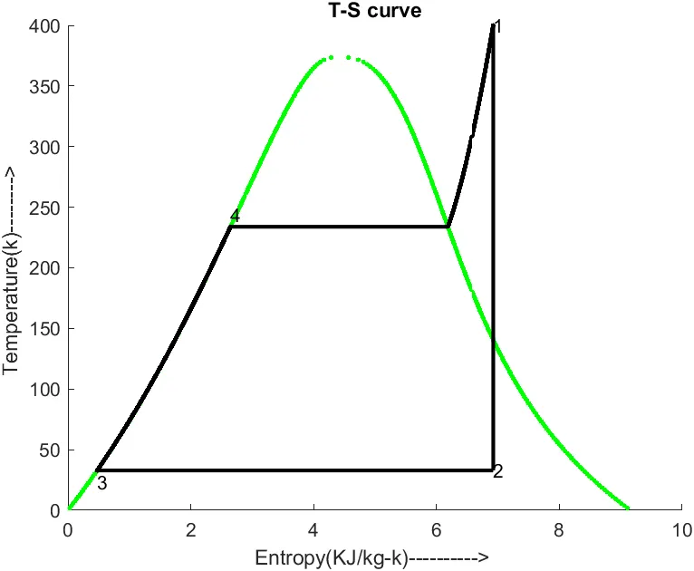
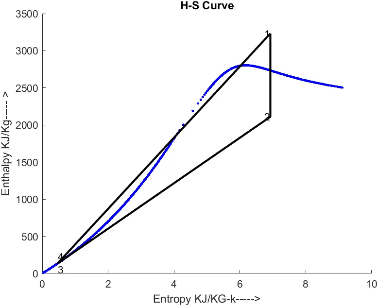
2. plot the corresponding T-s and h-s plots for the given set of inputs.
Theory-:
The Rankine cycle is an idealized thermodynamic cycle describing the process by which certain heat engines, such as steam turbines or reciprocating steam engines, allow mechanical work to be extracted from a fluid as it moves between a heat source and heat sink.
Heat energy is supplied to the system via a boiler where the working fluid (typically water) is converted to a high pressure gaseous state (steam) in order to turn a turbine. After passing over the turbine the fluid is allowed to condense back into a liquid state as waste heat energy is rejected before being returned to boiler, completing the cycle. Friction losses throughout the system are often neglected for the purpose of simplifying calculations as such losses are usually much less significant than thermodynamic losses, especially in larger systems.
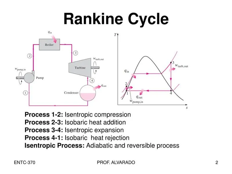
four major equipment in Rankine cycle -:
1.Boiler
2.Turbine
3.Condensor
4.Pump
Enthalpy-:In thermodynamics, the enthalpy is the measure of energy in a thermodynamic system. It is the thermodynamic quantity equivalent to the total heat content of a system. The enthalpy is defined to be the sum of the internal energy E plus the product of the pressure p and volume V. In many thermodynamic analyses the sum of the internal energy U and the product of pressure p and volume V appears, therefore it is convenient to give the combination a name, enthalpy, and a distinct symbol, H.
In thermodynamics, the enthalpy is a measurement of energy in a thermodynamic system. Enthalpy is equivalent to the total heat content of a system.
Entropy-: Entropy is a thermodynamic function that we use to measure uncertainty or disorder of a system. Moreover, the entropy of solid (particle are closely packed) is more in comparison to the gas (particles are free to move). Also, scientists have concluded that in a spontaneous process the entropy of process must increase.
Dryness Fraction -:The steam dryness fraction is used to quantify the amount of water within steam. If steam contains 10% water by mass, it's said to be 90% dry, or have a dryness fraction of 0.9.
Steam dryness is important because it has a direct effect on the total amount of transferable energy contained within the steam (usually just latent heat), which affects heating efficiency and quality.
For example, saturated steam (100% dry) contains 100% of the latent heat available at that pressure. Saturated water, which has no latent heat and therefore 0% dryness, will only contain sensible heat.
Isentropic compression (compression in centrifugal pumps) – The liquid condensate is compressed adiabatically from state 1 to state 2 by centrifugal pumps (usually by condensate pumps and then by feedwater pumps). The liquid condensatei s pumped from the condenser into the higher pressure boiler
The work required for the compressor is given by WPumps = H2 – H1.
Isobaric heat addition (in a heat exchanger – boiler) – In this phase (between state 2 and state 3) there is a constant-pressure heat transfer to the liquid condensate from an external source, since the chamber is open to flow in and out.The net heat added is given by Qadd = H3 – H2
Isentropic expansion (expansion in a steam turbine) – Steam from the boiler expands adiabatically from state 3 to state 4 in a steam turbine to produce work and then is discharged to the condenser (partially condensed).

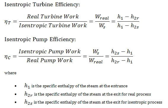
Required Inputs:
Turbine Inlet temperature = 400° C
Turbine Inlet Pressure = 30 bars
Turbine Outlet Pressure = 0.05 bars = Condenser Inlet Pressure
Matlab Program of Rankine Cycle Simulator:
close all
clear all
clc
disp('----------Rankine Cycle Simulator------------');
fprintf('\n')
disp('1-2 stage is isntropic expansion in turbine .')
disp('2-3 stage is constant pressure heat rejection by the condensor .')
disp('3-4 stage  is isentropic compression in pump work.')
disp('4-1 stage is constant pressure heat addition by the boiler.')
fprintf('\n')
P1=input('enter the initial pressure of steam in turbine( in bar)--:');
T1= input('enter the temperature at inlet of turbine (in Degee celcius) --:');
P2= input('enter the pressure at condensor(in bar)--:');
% calculation of steam state values
% getting 1_st state  point value from the XSteam Function
 H1=XSteam('h_pt',P1,T1);
 S1=XSteam('s_pt',P1,T1);
 H_L1=XSteam('hl_p',P1);
 H_G1=XSteam('hv_p',P1);
 S_L1=XSteam('sl_p',P1);
 S_G1=XSteam('sv_p',P1);
 T_sat1=XSteam('Tsat_p',P1);

 % getting 2_nd state point value from the XSteam Function
 S2=S1;
  H_L2=XSteam('hl_p',P2);
 H_G2=XSteam('hv_p',P2);
 S_L2=XSteam('sl_p',P2);
 S_G2=XSteam('sv_p',P2);
 D=(S2-S_L2)/(S_G2-S_L2);
 H2=H_L2+D*(H_G2-H_L2);
 T2=XSteam('T_ph',P2,H2);
 T_sat2=XSteam('Tsat_p',P2);

% 3_rd state point
P3=P2;
T3=T2;
H3=H_L2;
S3=S_L2;

% 4_th state point
P4=P1;
S4=S3;
T4=XSteam('T_ps',P4,S4);
H4=XSteam('H_ps',P4,S4);
% 5 th & 6th state piont
T5=XSteam('Tsat_p',P1);
T6=T5;
S5=XSteam('sL_p',P1);
S6=XSteam('sV_p',P1);
H5=XSteam('hL_p',P1);
H6=XSteam('hV_p',P1);

% Calculation of work Backworkratio,Specific Steam Conductivity & Efficiency
% Turbine Work
W_T=H1-H2;
% Pump work
W_P=H4-H3;
% Net work done
W_Net=W_T-W_P;
% thermal Efficiency of the Rankine cycle
Eff=(W_Net/(H1-H4))*100;
%Back Work Ratio
BWR=W_P/W_T;
%Specific Steam Conductivity
SSC=3600/W_T;
% Displaying all the Results
disp('--------------------Results--------------------');
% values display at state point 1
fprintf('\n\t\t\t\t')
disp('-------at state point 1');
fprintf('\n\t\t\t\tP1 is :- %.3f bar \n',P1)';
fprintf('\t\t\t\tT1 is :- %.3f Deg celcius \n',T1)';
fprintf('\t\t\t\tH1 is : %.3f KJ/kg \n ',H1);
fprintf('\t\t\t\tS1 is : %.3f KJ/kgk \n ',S1);
% values display at state point 2
disp('-------At state point 2');
fprintf('\nP2 is :- %.3f bar \n',P2)';
fprintf('T2 is :- %.3f Deg celcius \n',T2)';
fprintf('H2 is : %.3f KJ/kg \n ',H2);
fprintf('S2 is : %.3f KJ/kgk \n ',S2);
fprintf('x2 is -:%.3f \n',D)
% values display at state point 3
fprintf('\n\t\t\t')
disp('-------At state point 3');

fprintf('\n\t\t\tP3 is :- %.3f bar \n',P3)';
fprintf('\t\t\tT3 is :- %.3f Deg celcius \n',T3)';
fprintf('\t\t\tH3 is : %.3f KJ/kg \n ',H3);
fprintf('\t\t\tS3 is : %.3f KJ/kgk \n ',S3);
% values display at state point 4
disp('-------At state point 4');
fprintf('\nP4 is :- %.3f bar \n',P4)';
fprintf('T4 is :- %.3f Deg celcius \n',T4)';
fprintf('H4 is : %.3f KJ/kg \n ',H4);
fprintf('S4 is : %.3f KJ/kgk \n\n ',S4);
% Display tubine work
fprintf('turbine Work done-:%.3f KJ/kg \n',W_T);
fprintf('Pump Work done-:%.3f KJ/kg \n',W_P);
% net work done
fprintf('Net Work done-:%.3f KJ/kg \n',W_Net);
% Thermal efficiency
fprintf('Thermal Efficiency-:%f %',Eff);
% Specific  Steam Conductivity
fprintf('\nSpecific Steam Conductivity-:%.3f kg/kwh \n',SSC);
% Back Work Ratio
fprintf('Back Work Ratio-:%f  \n',BWR);
% plotting T-S Curve
t=linspace(0,373.5,200);
figure (1)
hold on
for i=1:length(t)
    plot(XSteam('sL_T',t(i)),t(i),'g.')
    plot(XSteam('sV_T',t(i)),t(i),'g.')
end
plot([S1 S2],[T1 T2],'LineWidth',2,'Color','k')
text(S1,T1,'1','FontSize',10)
 if D>1
     T3=T_sat2;
     plot([S2 S_G2 S3 S4],[T2 T_sat2 T3 T4],'LineWidth',2,'Color','k')
     T2=T_sat2;
     text(S2,T2,'2','FontSize',10)
     text(S3,T3,'3','FontSize',10)
 else
      plot([S2 S3 S4],[T2 T3 T4],'LineWidth',2,'Color','k')
     text(S2,T2,'2','FontSize',10)
     text(S3,T3,'3','FontSize',10,'HorizontalAlignment','left','VerticalAlignment','top')
 end
 n=linspace(T1,T2,500);
 for i=1:length(n)
    plot(XSteam('s_pT',P1,n(i)),n(i),'.','lineWidth',2,'Color','k')
 end
  plot([S_L1 S_G1],[T_sat1 T_sat1],'LineWidth',2,'Color','k')
  text(S_L1,T_sat1,'4','FontSize',10,'HorizontalAlignment','left','VerticalAlignment','bottom')
  xlabel('Entropy(KJ/kg-k)----------> ')
  ylabel('Temperature(k)--------> ')

  title('T-S curve')

% plotting H-S Curve
figure(2)
hold on
for i=1:length(t)
     plot(XSteam('sL_T',t(i)),XSteam('hL_T',t(i)),'b.')
    plot(XSteam('sV_T',t(i)),XSteam('hV_T',t(i)),'b.')
end
plot([S1 S2 S3 S4 S1],[H1 H2 H3 H4 H1],'LineWidth',2, 'Color','k')
text(S1,H1,'1','FontSize',10,'HorizontalAlignment','right')
text(S2,H2,'2','FontSize',10,'HorizontalAlignment','right')
text(S3,H3,'3 ','FontSize',10,'HorizontalAlignment','left','VerticalAlignment','top')
text(S4,H4,'4 ','FontSize',10,'HorizontalAlignment','left','VerticalAlignment','bottom')
xlabel('Entropy KJ/KG-k----->')
ylabel('Enthalpy KJ/Kg----- >')

title('H-S Curve')
output plots -: with titles
- Explanation-:The program begins with clear all close all clc to erase the workplace and command window.
- Ask for input variables p1,t1,p2 are given by input
- @state -1 values for enthalpy & entropy are extracted as afunction of pressure.& temperature.
- h_pt s_pt,hL_p,sv_p etc…are the default variables whose value is stored in XSteam file.
- Similarly ,all the variable for all state are extractedusing a suitable formate.
- Pressure , temperature enthalpy,entropy, for all state variables are extractedas a function of the dependent
- Variable from the XSteam file.
- @state 2 is a condenser inlet where the high pressures steam is converted into low-pressure water and hence dryness fraction enthalpy & entropy for saturated vapour & saturated water are considered to calculate the specific heat.
- @state3 the water is condense back to its saturation temperature and fed to pump this temperature of water at the exit of the condenser entry of the pump is the same.
- @ state 4 this is constant pressure heat addition hence pressure is equal to p1,but the temperature increases on heating at constant pressure & constant volume as our entropy remains same and hence Cp/Cv=gamma is consider as to find temperature T4.
- Define a two or more points 5 and 6 to plot cycle in detail.
- Finally work done and heat evolved & SSC are calculated by basic formula.
- To plot the saturation curve a temperature range is defined using linspace command and for the overall length of this temperature values of enthalpy & entropyare calculated at every temperature point the break in the saturation curve separates the liquid phase & vapour phase.
- Now all the necessary data is found out plotting is done for both T-s & H-S curve using the plot commands
- Annotation are assigned using text command.
- Result of the cycle simulation is displayed over command window using fprintf command.
Output Window- Display all content same as question want
MATLAB Command Window Page 1
----------Rankine Cycle Simulator------------
1-2 stage is isntropic expansion in turbine .
2-3 stage is constant pressure heat rejection by the condensor .
3-4 stage is isentropic compression in pump work.
4-1 stage is constant pressure heat addition by the boiler.
enter the initial pressure of steam in turbine( in bar)--:30
enter the temperature at inlet of turbine (in Degee celcius) --:400
enter the pressure at condensor(in bar)--:0.05
--------------------Results--------------------
                    -------at state point 1
                    P1 is :- 30.000 bar
                    T1 is :- 400.000 Deg celcius
                    H1 is : 3231.571 KJ/kg
                    S1 is : 6.923 KJ/kgk
 -------At state point 2
P2 is :- 0.050 bar
T2 is :- 32.875 Deg celcius
H2 is : 2110.708 KJ/kg
S2 is : 6.923 KJ/kgk
x2 is -:0.814
                    -------At state point 3
                    P3 is :- 0.050 bar
                    T3 is :- 32.875 Deg celcius
                    H3 is : 137.765 KJ/kg
                    S3 is : 0.476 KJ/kgk
 -------At state point 4
P4 is :- 30.000 bar
T4 is :- 32.945 Deg celcius
H4 is : 140.762 KJ/kg
S4 is : 0.476 KJ/kgk

turbine Work done-:1120.863 KJ/kg
Pump Work done-:2.997 KJ/kg
Net Work done-:1117.866 KJ/kg
Thermal Efficiency-:36.167417
Specific Steam Conductivity-:3.212 kg/kwh
Back Work Ratio-:0.002674
Workplace-
MATLAB Workspace Page 1
Jun 5, 2022 5:23:35 PM
Name        Value
ans         29
BWR         0.0027
D           0.8143
Eff         36.1674
H1          3.2316e+03
H2          2.1107e+03
H3          137.7651
H4          140.7622
H5          1.0084e+03
H6          2.8033e+03
H_G1        2.8033e+03
H_G2        2.5608e+03
H_L1        1.0084e+03
H_L2        137.7651
i           200
n          1x500 double
P1          30
P2         0.0500
P3         0.0500
P4          30
S1         6.9233
S2         6.9233
S3         0.4763
S4         0.4763
S5         2.6456
S6         6.1858
S_G1       6.1858
S_G2       8.3939
S_L1       2.6456
S_L2       0.4763
SSC        3.2118
t          1x200 double
T1         400
T2        32.8755
T3        32.8755
T4        32.9452
T5        233.8584
T6        233.8584
T_sat1    233.8584
T_sat2    32.8755
W_Net     1.1179e+03
W_P        2.9971
W_T        1.1209e+0
References -: www.google.com
Specific Steam Consumption - an overview | ScienceDirect Topics
What is Rankine Cycle - Steam Turbine Cycle - Definition (thermal-engineering.org)