Project 2 - Rankine cycle Simulator

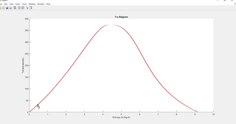
clear all 
close all 
clc

% Creating Rankine Cycle Simulator 
disp('RANKINE CYCLE SIMULATOR') 
disp('1-2 : Isentropic Expansion in the Turbine') 
disp('2-3 : Isobaric Heat Rejection by the Condenser') 
disp('3-4 : Isentropic Compression in the Pump') 
disp('4-1 : Isobaric Heat Addition by the Boiler') 
disp(' ')

t = linspace(0,373.15,300);

% Inputs to be specified 
P1 = input('Enter the Pressure at the Turbine Inlet (in bar): ');
T1 = input('Enter the Temperature at the Turbine Inlet (in Degree Celsius): ');
P2 = input('Enter the Pressure at the Condenser (in bar): ');
disp(' ')

% State Point 1 
h1 = XSteam('h_pT',P1, T1); 
s1 = XSteam('s_pT',P1, T1); 
h_l1 =XSteam('hL_p',P1); 
h_g1 =XSteam('hv_p',P1);
s_l1 =XSteam('sl_p',P1); 
s_g1 =XSteam('sv_p',P1); 
T_sat1=XSteam('Tsat_p',P1); 


% State Point 2 
s2 = s1; 
s_l2 = XSteam('sL_p',P2); 
s_g2 = XSteam('sV_p',P2);

% Dryness Fraction 
x = (s2 - s_l2)/(s_g2 - s_l2);

h_l2 = XSteam('hL_p',P2);
h_g2 = XSteam('hV_p',P2);
h2 = h_l2 + x*(h_g2 - h_l2);
T2 = XSteam('T_ph',P2, h2);
T_sat2 = XSteam('Tsat_p',P2);

% State Point 3 
h3 = h_l2;
s3 = s_l2;
P3 = P2;
T3 = T2;

% State Point 4 
s4 = s3;
P4 = P1;
h4 = XSteam('h_ps',P4, s4);
T4 = XSteam('T_ps',P4,s4);

% plotting

% T-s Diagram 
figure(1), clf 
hold on 

% Saturation curve
for i = 1:length(t)
plot(XSteam('sL_T',t(i)),t(i),'r.')
plot(XSteam('sv_T',t(i)),t(i),'r.')
end

% Rankine Cycle
plot([s1 s2],[T1 T2], 'linewidth',2,'color','g')
text(s1,T1,'1','Fontsize',15)

% Beyond saturation curve
if x > 1
T3 = T_sat2;
plot([s2 s_g2 s3 s4],[T2 T_sat2 T3 T4], 'linewidth',2,'color','g')
text(s1,12,'2', 'Fontsize',15)
text(s3,T3,'3','FontSize',15,'HorizontalAlignment','left','VerticalAlignment','top')

% Beneath saturation curve 
else
plot([s2 s3 s4],[T2 T3 T4],'linewidth',2,'color','g')
text(s1,T2,'2','Fontsize',15)
text(s3,T3,'3','Fontsize',15,'HorizontalAlignment','left','verticalAlignment', 'top')
end

n = linspace(T1, T2,500); 
for i = 1:length(n)
plot(XSteam('s_pT',P1,n(i)),n(i),'.','linewidth',2,'color','g')
end 


plot([s_l1 s_g1],[T_sat1 T_sat1],'linewidth',2,'color','g')
text(s_l1,T_sat1, '4','FontSize',15,'VerticalAlignment','bottom') 
xlabel('Entropy (kJ/kg-K)') 
ylabel('Temperature(k)') 
title('T-s Diagram')

% h-s Diagram
figure(2), clf
hold on

% Saturation curve 
for i = 1:length(t)
plot(XSteam('sL_T',t(i)),XSteam('hL_T',t(i)),'r.')
plot(XSteam('sV_T',t(i)),XSteam('hV_T',t(i)), 'r.')
end

% Rankine Cycle
plot([s1 s2 s3 s4 s1],[h1 h2 h3 h4 h1], 'linewidth',2,'color','g') 
text(s1,h1,'1','Fontsize',15)
text(s2,h2,'2','FontSize',15)
text(s3,h3,'3','Fontsize',15)
text(s4,h4+90,'4','FontSize',15)

xlabel('Entropy (kJ/kg-K)') 
ylabel ('Enthalpy (kJ/kg)')
title('h-s Diagram')

% Calculation of desired quantities 

 %Work done by turbine
 W_t = h1 - h2;

 %Work done by pump 
 W_p = h4 - h3;

 %Net work done 
 W_net = W_t - W_p;

 %Thermal efficiency
 n_thermal = (1 - ((h2 - 13)/(h1 - h4)))*100;
%Back work ratio 

BWR = W_p/W_t;

%Specific Steam Conductivity 
SSC = 3600/W_t;

% Displaying results in command window
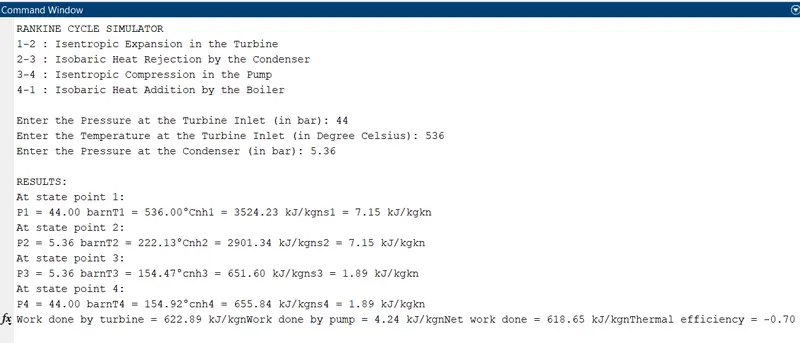
disp('RESULTS:')

disp('At state point 1: ') 
fprintf('P1 = %.2f barn',P1)
fprintf(['T1 = %.2f' char(176) 'Cn'],T1)
fprintf('h1 = %.2f kJ/kgn',h1)
fprintf('s1 = %.2f kJ/kgkn',s1)
disp(' ')

disp('At state point 2: ')
fprintf('P2 = %.2f barn',P2)
fprintf(['T2 = %.2f' char(176) 'Cn'],T2)
fprintf('h2 = %.2f kJ/kgn', h2)
fprintf('s2 = %.2f kJ/kgkn', s2) 
disp(' ')

disp('At state point 3: ')
fprintf('P3 = %.2f barn',P3)
fprintf(['T3 = %.2f' char(176) 'cn'],T3) 
fprintf('h3 = %.2f kJ/kgn',h3)
fprintf('s3 = %.2f kJ/kgkn', s3)
disp(' ')

disp('At state point 4: ') 
fprintf('P4 = %.2f barn',P4)
fprintf(['T4 = %.2f' char(176) 'cn'],T4)
fprintf('h4 = %.2f kJ/kgn', h4) 
fprintf('s4 = %.2f kJ/kgkn', s4)
disp(' ')

fprintf('Work done by turbine = %.2f kJ/kgn', W_t)
fprintf('Work done by pump = %.2f kJ/kgn', W_p)
fprintf('Net work done = %.2f kJ/kgn', W_net)
fprintf('Thermal efficiency = %.2f %%', n_thermal)
fprintf('Back-work ratio = %fn', BWR)
fprintf('Specific Steam Conductivity = %.2f kg/kwhn',SSC) 

EXPLANATION OF CODE:

1.Start the program with clear all,close all,clc.

then create the rankine simulator by using disp command for all the processes

give t=linspace(0,373.15,300)

give the inputs at state point one as was given in the challenge

also give the same at state point 2,3,4 also

and give

and for desired results we use disp for state point 1