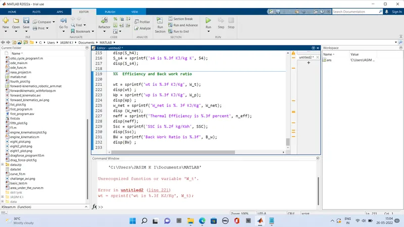
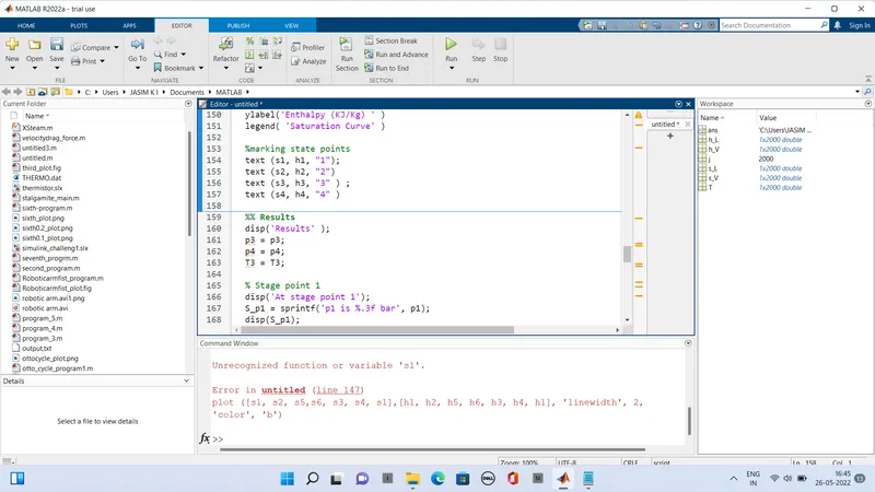
%% Rankine Cycle Simulation using Matlab

% Taking the Thermal properties using Xsteam data file
% To calculate the work done by turbine, pump, net workdone, efficiency
clear all
close all
clc

%% Rankine Cycle Process

%Process 1-2 is Isentropic Expansion ( Turbine )
% Process 2-3 is Constant Pressure heat reduction ( Condensor )
%Process 3-4 is Isentropic Compression ( Pump )
% Process 4-1 is Constant pressure Heat addition ( boiler )

% displaying the process of Rankine cycle
disp( 'Rankine Cycle Process' )
disp('Process 1-2 is Isentropic Compression in Turbine' )
disp('process 2-3 is Constant pressure Heat reduction in the Condensor' )
disp( 'process 3-4 is Isentropic Expansion in Pump')
disp( 'Process 4-1 is Constant Pressure heat addition in Boiler' )


%% Inputs

% Inputs pressure is taken in 'bar', Temperature is taken in 'degree Celcius'
% values of pressure and temperature.

T3 = input( 'Inlet Temperature for Turbine T3(C) = ')
p3 = input('Inlet Pressure of the Turbine p3(bar) = ')
p4 = input('Outlet Pressure of the Turbine p4(bar) = ')

%% State_Points

% by using XSteam library we are taking the required data like pressure, temperature, entropy, enthalpy

% State 1 Inputs

T1 = XSteam( 'Tsat_p' , p4);
p1 = p4;
h1 = XSteam( 'hL_p' , p4);
s1 = XSteam( 'sL_p' , p4);


% State_2 Inputs


T2 = XSteam( 'Tsat_p' , p3, s1);
p2 = p3;
h2 = XSteam( 'h_ps' , p3, s1);
s2 = s1;


% State 3 Inputs

h3 = XSteam( 'h_pT' , p3, T3);
s3 = XSteam( 's_pT' , p3, T3);


% State_4 Inputs
sg4 = XSteam('sV_p', p4)-XSteam('sL_p', p4);
hg4 = XSteam('hV_p', p4)-XSteam('hL_p', p4);
s4 = s3;
X = (s4-s1)/sg4;
h4 = h1+(X*hg4);
v4 = XSteam( 'VL_p', p4);
T4 = XSteam( 'T_ph' , p4, h4);


%Intermediate State points

T5 = XSteam( 'Tsat_p', p3);
h5 = XSteam( 'hL_p' , p3);
s5 = XSteam( 'sL_p' , p3);
T6 = XSteam( 'Tsat_p' , p3);
h6 = XSteam( 'hv_p', p3);
s6 = XSteam( 'sV_p' , p3);
P5 = p3;
p6 = p3;

%% calculating work done

% workdone by Turbine
W_t = h3-h4;

% workdone by Pump
W_p = v4*(p3 -p4)*100;
hf2 = W_p + h1;

% Calculating Net workdone
W_net = W_t-W_p;

%% Calculating Heat in to the system
Q_in = h3-h2;

%% Calculating Thermal Efficiency
n_eff = (W_net/Q_in)*100;

%% Calculating specific steam consumption (SSC) = mass flow rate/net workdone
SSC = (3600/W_net);

%% Calculating Back Work Ratio
B_w = (W_p/W_t);


%% Plot for the Saturation Curve

S = linspace(0.1,10, 1000);
for i = 1: length(S)
Tsat (i) = XSteam('Tsat_s' ,S(i));
end

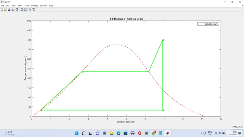
%% Plotting T-S diagram

figure(1)
plot (S, Tsat, ' -- ', 'Linewidth', 1, 'color', 'r')
hold on
plot ( [ s1, s5, s5, s6, s3, s4, s1], [T1, T2, T5, T6, T3, T4, T1], 'linewidth' , 2, 'color' , 'g')
xlim([0 10])
ylim([0 500])
title('T-S Diagram of Rankine Cycle')
xlabel( 'Entropy, s(Kj/kgk) ' )
ylabel ( ' Temperature (degree c)')
legend( 'saturation curve' )
hold off

% marking State points
text (s1, T1, "1");
text (s5, T2, "2");
text (s3, T3, "3");
text (s4, T4, "4") ;


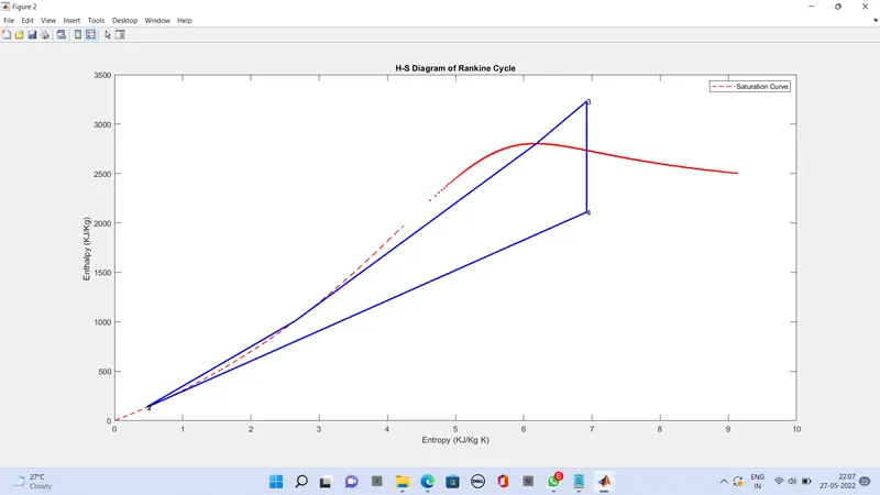
%% Plotting H_S diagram
T = (1:2000);
for j = 1: length(T)
h_L(1,j) = XSteam('hL_T' , j);
h_V(1, j) = XSteam('hV_T' , j);
s_L(1, j) = XSteam('sL_T', j);
s_V(1,j) = XSteam('sV_T', j);
end

figure(2)
plot (s_L, h_L, '--', 'Linewidth',1, 'color' , 'r')
hold on
plot (s_V, h_V, '.', 'Linewidth', 1, 'color', 'r')
plot ([s1, s2, s5,s6, s3, s4, s1],[h1, h2, h5, h6, h3, h4, h1], 'linewidth', 2, 'color', 'b')
title('H-S Diagram of Rankine Cycle' )
xlabel('Entropy (KJ/Kg K)' )
ylabel('Enthalpy (KJ/Kg) ' )
legend( 'Saturation Curve' )

%marking state points
text (s1, h1, "1");
text (s2, h2, "2")
text (s3, h3, "3" ) ;
text (s4, h4, "4" )

%% Results
disp('Results' );
p3 = p3;
p4 = p4;
T3 = T3;

% Stage point 1
disp('At stage point 1');
S_p1 = sprintf('p1 is %.3f bar', p1);
disp(S_p1);
S_T1 = sprintf('T1 is %.3f "c', T1);

disp(S_T1);
S_h1 = sprintf('h1 is %.3f <3/kg', h1);
disp (S_h1) ;
S_s1 = sprintf('s1 is %.3f KJ/kg K', s1);
disp(S_s1) ;

% Stage point 2
disp('At stage point 2') ;
S_p2 = sprintf('p2 is %. 3f bar' , p2);
disp(S_p2);
S_T2 = sprintf('T2 is X.3f C', T2);
disp(S_T2);
S_h2 = sprintf('h2 is %.3f KJ/Kg', h2);
disp(S_h2) ;
S_s2 = sprintf('s2 is X.3f K3/Kg K', s2);
disp(S_s2);


% Stage point3

disp('At stage point 3');
S_p3 = sprintf('p3 is %.3f bar', p3);
disp(S_p3) ;
S_T3 = sprintf('13 is %.3f C', T3);
disp(S_T3) ;
S_h3 = sprintf('h3 is %.3f KJ/kg', h3);
S_T3 = sprintf('T3 is %.3f C', 13);
disp(S_T3);
S_h3 = sprintf('h3 is %. 3f <3/kg', h3);
disp(S_h3);
S_s3 = sprintf('s3 is %.3f KJ/kg K', s3);
disp(S_s3);


% Stage point 4
disp('At stage point 4');
S_p4 = sprintf('p4 is %.3f bar', p4);
disp(S_p4);
S_T4 = sprintf('T4 is %.3f C', 14);
disp(S_T4);
S_h4 = sprintf('h4 is %.3f KJ/kg', h4);
disp(S_h4);
S_s4 = sprintf('s4 is %.3f KJ/kg K', 54);
disp(S_s4);

%%  Efficiency and Back work ratio

wt = sprintf('wt is %.3f KJ/Kg', W_t);
disp(wt) ;
Wp = sprintf('wp is %.3f KJ/Kg', W_p);
disp(Wp) ;
w_net = sprintf('W_net is %. 3f KJ/Kg', W_net);
disp (W_net);
neff = sprintf('Thermal Efficiency is %.3f percent', n_eff);
disp(neff);
Ssc = sprintf('SSC is %.2f kg/KWh', SSC);
disp(Ssc);
BW = sprintf('Back Work Ratio is %.3f', B_w);
disp(BW) ;
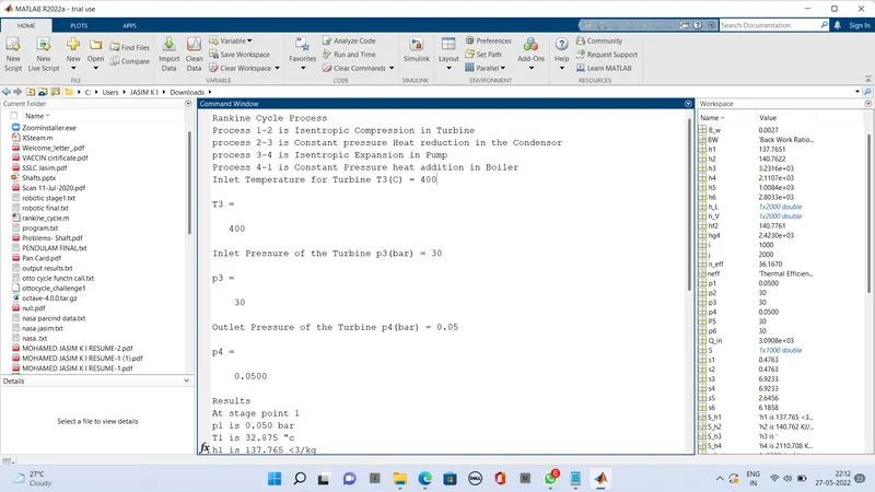
Rankine Cycle Process
Process 1-2 is Isentropic Compression in Turbine
process 2-3 is Constant pressure Heat reduction in the Condensor
process 3-4 is Isentropic Expansion in Pump
Process 4-1 is Constant Pressure heat addition in Boiler
Inlet Temperature for Turbine T3(C) = 400

T3 =

   400

Inlet Pressure of the Turbine p3(bar) = 30

p3 =

    30

Outlet Pressure of the Turbine p4(bar) = 0.05

p4 =

    0.0500

Results
At stage point 1
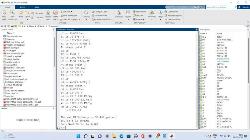
p1 is 0.050 bar
T1 is 32.875 "c
h1 is 137.765 <3/kg
s1 is 0.476 KJ/kg K
At stage point 2
p2 is
T2 is X.3f C
h2 is 140.762 KJ/Kg
s2 is X.3f K3/Kg K
At stage point 3
p3 is 30.000 bar
13 is 400.000 C
T3 is 13.000 C
h3 is
s3 is 6.923 KJ/kg K
At stage point 4
p4 is 0.050 bar
T4 is 14.000 C
h4 is 2110.708 KJ/kg
s4 is 54.000 KJ/kg K
wt is 1120.863 KJ/Kg
wp is 3.011 KJ/Kg
   1.1179e+03

Thermal Efficiency is 36.167 percent
SSC is 3.22 kg/KWh
Back Work Ratio is 0.003
>>