Project 2 - Rankine cycle Simulator
Aim-
- To Simulate a Rankine cycle using matlab.
- Extracting Steam and water properties from Xstram file.
- Calculating all the state points of the cycle based on User inputs.
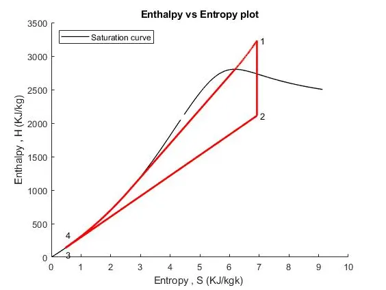
- Plotting the T vs S and H vs S plot for the given input.
Theory- A rankine cycle is a romanticized Thermodynamic cycle which oversees the working of a Heat Engine. In Rankine cycle,the rubbing misfortunes of an intensity motor are dismissed. It is a cycle which converts heat into mechanical energy which for the most part is changed over into electrical energy . There are four parts in this cycle which work on four different processes.The four parts are turbine,Condensor,Pump and Boiler. Rankine cycle is only a change of Carnot cycle. Ideal Rankine cycle is exceptionally valuable in steam power plants and internal combustion plants. To work on the proficiency of Rankine cycle in the steam power plant, there are a few changes in Rankine cycle which contrasts from the Carnot cycle. A siphon, first and foremost, is utilized instead of condenser to deal with fluid, rather than a combination of fluid and vapour.Secondly, exhaust steam from the turbine is totally consolidated in the condenser, find in the accompanying outline:
Processes and Working :
There are four processes in the rankine cycle :
- Process 1-2 : Isentropic Expansion in the turbine
- Process 2-3 : Constant pressure Heat rejection in condenser
- Process 3-4 : Isentropic compression in the pump
- Process 4-1 : Constant pressure heat addition in the boiler
Rankine cycle efficiency ηR is -

Back Work Ratio:
The fraction of the work produced by the turbine that is consumed by the compressor.
BW ratio=Wp/Wt
MATLAB PROGRAM FOR RANKINE CYCLE SIMULATOR
clear all
close all
clc
disp(' RANKINE CYCLE ');
disp('1-2 is Constant pressure heat addition in the boiler');
disp('2-3 is Isentropic Expansion in the Turbine');
disp('3-4 is Constant pressure heat removal in the Condenser');
disp('4-1 is Isentropic compression in the pump');
p1 = input('nValue of pressure at turbine inlet, p1(in bar) = ');
T1 = input('nValue of temperature at turbine inlet, T1(in degree.C) = ');
p2 = input('nValue of pressure at condenser inlet, p2(in bar) = ');
% At State 1
h1 = XSteam('h_pT', p1, T1); % Extracting Enthalpy at state pt 1
s1 = XSteam('s_pT', p1, T1); % Similarly
% At State 2
s2 = s1; % Isentropic Expansion
sf2= XSteam('sL_p', p2); % Saturated Liquid Entropy
sg2 = XSteam('sV_p', p2); % Saturated Vapour Entropy
x2 = (s2-sf2)/(sg2-sf2);
hf2 = XSteam('hL_p', p2);
hg2 = XSteam('hV_p', p2);
h2 = hf2 + (x2*(hg2-hf2));
% At State 3
p3 = p2; % Constant pressure Heat rejection in Condenser
s3= XSteam('sL_p', p3);
h3 = XSteam('hL_p', p3);
% At State 4
s4 = s3;
p4 = p1;
% Work done by turbine
Wt = h1 - h2;
% Work done to run pump
v3 = XSteam('vL_p', p3);
Wp = v3*(p4 - p3)*100;
h4 = h3 + Wp;
%Net work
Wnet = Wt - Wp;
%Heat into the system
Qin = h1 - h4;
%Heat out of the system
Qout = h2 - h3;
%Thermal efficiency
thermal_eff = (Wnet/Qin)*100;
%Specific Steam Consumption
%SSC = mass flow rate/power
SSC = (3600/Wnet);
% Back Work ratio
BW = (Wp/Wt)
% Calculation of Temperatures at the state points
T3 = XSteam('Tsat_p', p3);
T2 = T3;
Cp4 = XSteam('Cp_ps', p4, s4);
Cv4 = XSteam('Cv_ps', p4, s4);
k = Cp4/Cv4;
T4 = T3/((p3/p4)^((k-1)/k));
%Calculating Temperature, Entropy and Enthalpy at the vapour and liquid line for plotting
T6 = XSteam('Tsat_p', p1);
s5 = XSteam('sL_p', p1);
s6 = XSteam('sV_p', p1);
h5 = XSteam('hL_p', p1);
h6 = XSteam('hV_p', p1);
T5 = T6;
%Plotting the saturation curve
T = linspace(1,375,1000);
for i = 1:length(T)
sf(i) = XSteam('sL_T', T(i));
sg(i) = XSteam('sV_T', T(i));
hf(i) = XSteam('hL_T', T(i));
hg(i) = XSteam('hV_T', T(i));
end
%Plotting T-s diagram
figure(1)
hold on
plot(sf, T, 'r','linewidth',1)
plot(sg, T, 'r','linewidth',1)
plot([s1 s2], [T1 T2], 'b', 'linewidth', 2)
plot([s2 s3], [T2 T3] ,'b', 'linewidth', 2)
plot([s3 s4], [T3 T4], 'b', 'linewidth', 2)
plot([s4 s5], [T4 T5], 'b', 'linewidth', 2)
plot([s5 s6], [T5 T6], 'b', 'linewidth', 2)
sc1 = linspace(s6, s1, 1000);
for l = 1:length(sc1)
Tc1(l) = XSteam('T_ps', p1, sc1(l));
end
plot(sc1, Tc1, 'b', 'linewidth', 2)
text(s1+0.1, T1, '1')
text(s2+0.1, T2, '2')
text(s3, T3-20, '3')
text(s4, T4+20, '4')
title('Temp vs Entropy plot')
xlabel('Entropy ,S (Kj/kgk')
ylabel('Temperature (degree C) ')
legend('Saturation curve')
%Plotting h-s diagram
figure(2)
hold on
plot(sf, hf, 'k', 'linewidth', 1)
plot(sg, hg, 'k', 'linewidth', 1)
plot([s1 s2], [h1 h2], 'r', 'linewidth', 2)
plot([s2 s3], [h2 h3], 'r', 'linewidth', 2)
plot([s3 s4], [h3 h4], 'r', 'linewidth', 2)
hc = linspace(h4, h5, 100);
for r = 1:length(hc)
sch(r) = XSteam('s_ph', p1, hc(r));
end
plot(sch,hc, 'r', 'linewidth', 2)
plot([s5 s6], [h5 h6], 'r', 'linewidth', 2)
for m = 1:length(sc1)
hc1(m) = XSteam('h_ps', p1, sc1(m));
end
plot(sc1, hc1, 'r', 'linewidth', 2)
text(s1+0.1, h1, '1')
text(s2+0.1, h2, '2')
text(s3, h3-100, '3')
text(s4, h4 +200, '4')
title('Enthalpy vs Entropy plot')
xlabel('Entropy , S (KJ/kgk) ')
ylabel('Enthalpy , H (KJ/kg)')
legend('Saturation curve','location','northwest')
% Displaying the Results in the Command Window:
disp('Results');
p1 = p1;
T1 = T1;
p2 = p2;
disp('At stage point 1');
n1 = sprintf('P1 is %.3f bar',p1);
disp(n1);
n2 = sprintf('T1 is %.3f C',T1);
disp(n2);
n3 = sprintf('h1 is %.3f kJ/kg',h1);
disp(n3);
n4 = sprintf('s1 is %.3f kJ/kgK',s1);
disp(n4);
disp('At stage point 2');
n11 = sprintf('P2 is %.3f bar',p2);
disp(n11);
n21 = sprintf('T2 is %.3f C',T2);
disp(n21);
n31 = sprintf('h2 is %.3f kJ/kg',h2);
disp(n31);
n41 = sprintf('s2 is %.3f kJ/kgK',s2);
disp(n41);
disp('At stage point 3');
n12 = sprintf('P3 is %.3f bar',p3);
disp(n12);
n22 = sprintf('T3 is %.3f C',T3);
disp(n22);
n32 = sprintf('h3 is %.3f kJ/kg',h3);
disp(n32);
n42 = sprintf('s3 is %.3f kJ/kgK',s3);
disp(n42);
disp('At stage point 4');
n13 = sprintf('P4 is %.3f bar',p4);
disp(n13);
n23 = sprintf('T4 is %.3f C',T4);
disp(n23);
n33 = sprintf('h4 is %.3f kJ/kg',h4);
disp(n33);
n43 = sprintf('s4 is %.3f kJ/kgK',s4);
disp(n43);
n14 = sprintf('Wt is %.3f kJ/kg',Wt);
disp(n14);
n15 = sprintf('Wp is %.3f kJ/kg',Wp);
disp(n15);
n16 = sprintf('Wnet is %.3f kJ/kg',Wnet);
disp(n16);
n17 = sprintf('Thermal_efficiency is %.2f Percent',thermal_eff);
disp(n17);
n18 = sprintf('SSC is %.2f kg/kWh',SSC);
disp(n18);
n19 = sprintf('Back work ratio is %.3f ',BW);
disp(n19);
Explanation of Program
- Xsteam information is utilized to remove steam and water properties of enthaly , entropy at explicit tension and temperatures for sat fluid, sat fume conditions and so on .
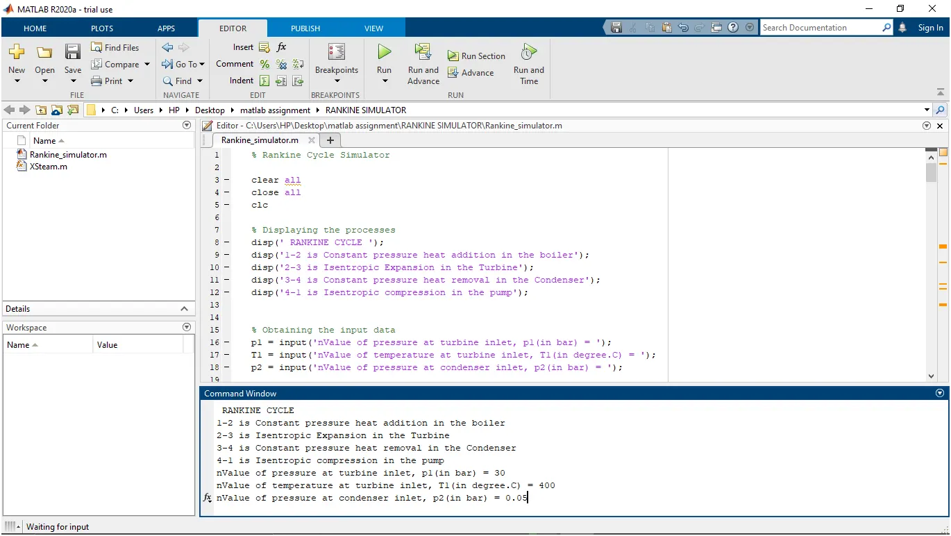
The program requires the contribution of Pressure ( in bar) at state point 1 ( turbine bay) , Temperature at same point (degree celcius) and tension at condenser channel (point 2).
With the assistance of these gulfs and from Xsteam information, the program computes all the state points of the Rankine cycle .
The Xsteam information fills in as , h1 = XSteam('h_pT' , p1 , T1) it returns the enthalpy of water at given tension and temperature in bar and degC separately.
As we extricate the information , we utilize thermodynamic connection to additional find state focuses and separate their information from XSteam which are referenced subsequent to concentrating on the Rankine cycle.
Sf and sg , hf and hg , where f and g represents soaked fluid and immersed fume separately are calculayed subsequent to concentrating on the plots of Rankine cycles and extricating information from Xsteam document.
The net work , work done by turbine , work done to run the siphon , Heat in and heat out are determined utilizing standard thermodynamic connection
Proficiency and Specific steam utilization (s.s.c) of the Rankine cycle is determined from thermodynamic relations and referencing them in program utilizing relations.
T , s and h are extricated at fume and fluid line for plotting reason , after fourth point for the variety you see in the plot .
Immersion bend is plotted in red for immersed fluid and soaked gas in T-S and in H-S it is dark .
Plot of T versus s and h versus s is made from every one of the focuses got from the program utilizing the plot order and referencing all the lables, linewidth, variety and title.
The plot changes as the client input changes for the previously mentioned inputs .
Results are shown in the order window by utilizing run order .
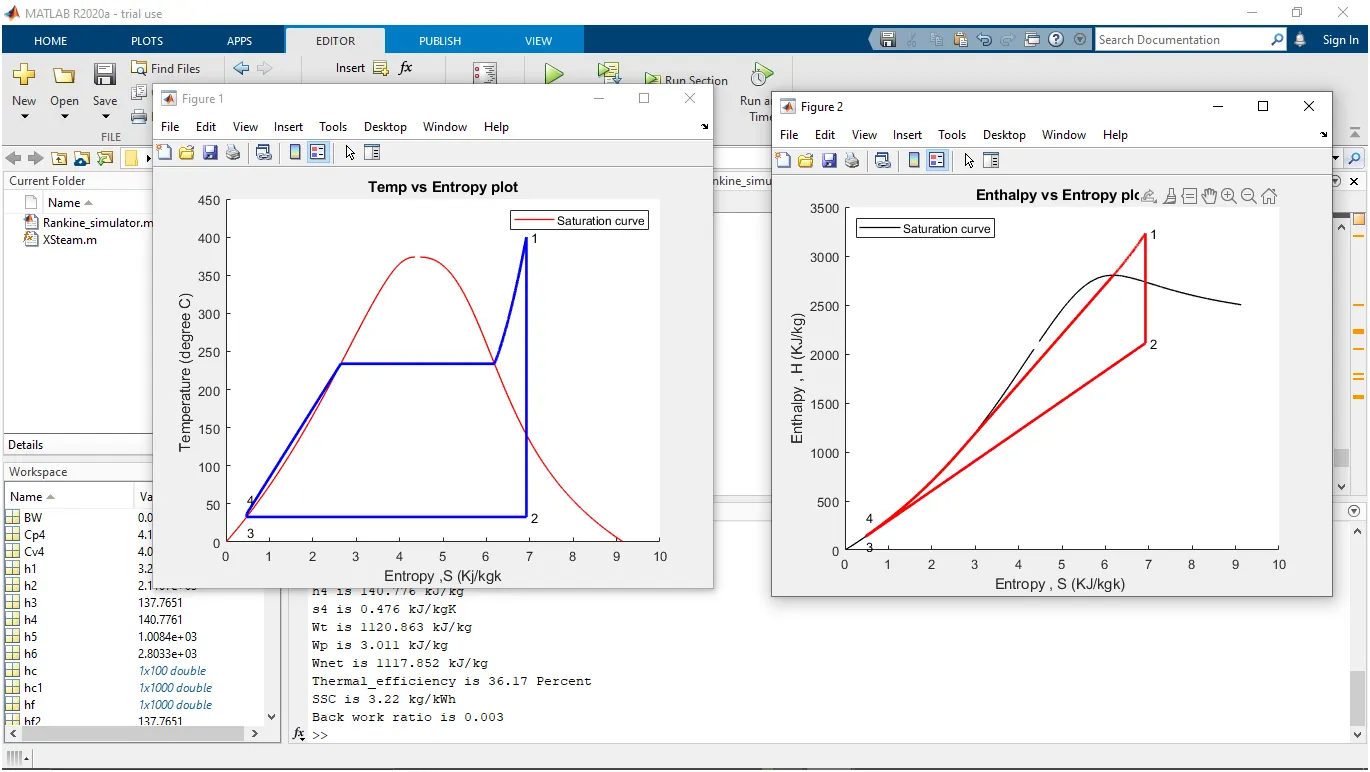
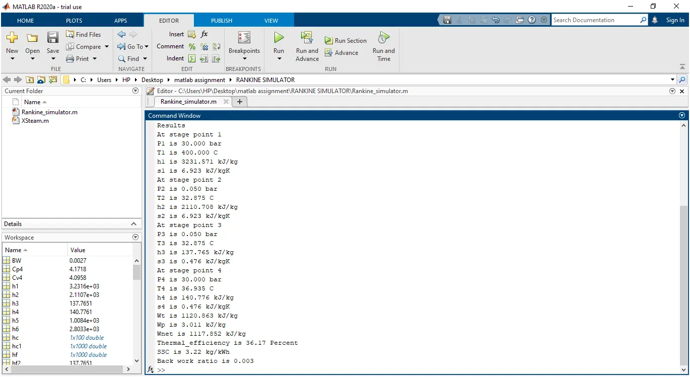
Result - The input, ouput screen and the various state points with various parameters generated in the command window are shown below
RESULTS and PLOTS
The performance of the Heat Engine was calculated and the following Observations were made:
- Net Work = 1120.863kJ/kg
- Thermal Efficiency = 36.17%
- Back Work Ratio = 0.003
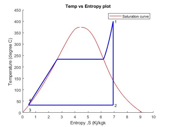
The T-S and H-S performance curves of the Rankine Cycle were plotted.
REFERENCES