Project 2 - Rankine cycle Simulator

Rankine Cycle - Basic process description

The Rankine cycle is the fundamental operating cycle of all power plants where an operating fluid is continuously evaporated and condensed. The selection of operating fluid depends mainly on the available temperature range.The Rankine cycle is an idealized thermodynamic cycle of a constant pressure heat engine that converts part of heat into mechanical work. In this cycle, the heat is supplied externally to a closed loop, which usually uses water (in a liquid and vapor phase) as the working fluid.

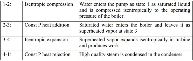
In an ideal Rankine cycle, the system executing the cycle undergoes a series of four processes: two isentropic (reversible adiabatic) processes alternated with two isobaric processes

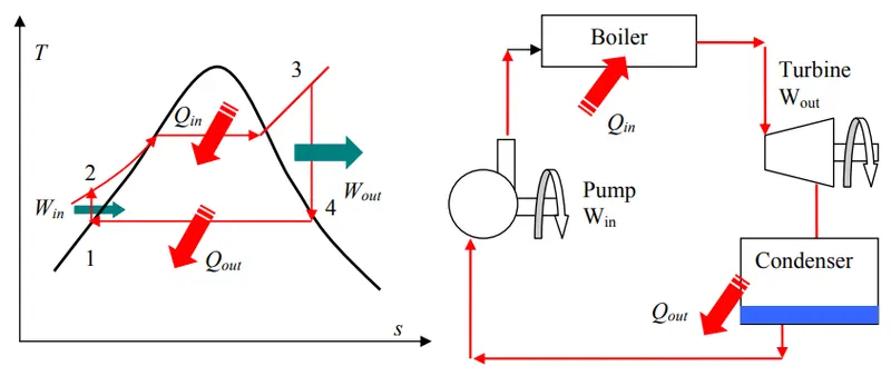
• Boiler is used to convert the water into steam according to the turbine’s desired temperature and pressure.
• Pump is a device which uses to transfers the water from one area to another high area. The pump also transfers the water from the reservoir or other water source into the boiler.
• Condenser cools the steam, converts it into liquid form, and sends this water back into the boiler.
• Steam Turbine will rotate the shaft of the generator to produce electricity. The turbine extracts the mechanical power from the steam and sends it into the condensate.

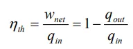
Thermal Efficiency: The thermal efficiency, η_th, represents the fraction of heat, Q_H, converted to work. Since energy is conserved according to the first law of thermodynamics and energy cannot be converted to work completely, the heat input, Q_H, must equal the work done, W, plus the heat that must be dissipated as waste heat Q_C into the environment.

The stages of completing a Rankine cycle are given below:

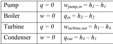
1. Isentropic Compression (1 to 2): In this stage, a pump uses to transfer the water or other working medium from the water body (canal or tank etc.) into the boiler. The pump requires a small amount of energy for initial pumping. It pumps the fluid by increasing the pressure of the fluid, but fluid entropy remains the same. For initial pumping, the work done on the pump is given below:
2. Constant Pressure Heat Addition Process (2 to 3): As the water is delivered into the boiler, an external heat source provides heat to the boiler. The boiler heated the water at constant pressure and converts it into dry saturated vapour (steam). During this process, the enthalpy of the liquid changes, and pressure remains constant.
3. Isentropic Expansion (3 to 4): After the constant pressure heat addition process, the steam enters into the turbine area, where it expands. As the steam expands, it strikes with the turbine blades, which convert the thermal energy of the steam into rotational energy (mechanical work). As the turbine blades are rotated, they also rotate a crankshaft that further rotates the coil of the generator. As the coil rotates in a magnetic field, it produces electricity. During this whole process, the pressure and temperature of the steam decrease; due to that, some condensation can happen.
4. Constant Pressure Heat Rejection Process (4 to 1): The vapour or steam enters the condenser tank after the expansion process. In this condensation process, the vapour is condensed to convert it into saturated liquid. During this process, the vapour rejects heat, but its liquid pressure remains the same.

Program Description:

Step 1: %cleaning command script- close all will closes all open MATLAB figure window, clear all will clear all data stored to a variable and the command clc will clear the command window.

Step 2: fprintf was used to display the process in command window as per the required output screen provided. \n is the command used to create a new line.

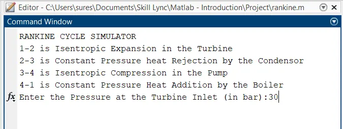
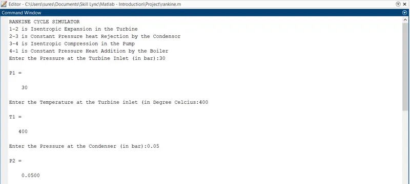
Step 3: "input" command is used to enter the values of turbine inlet pressure, turbine inlet temperature and pressure at the condenser.

Step 4: In the next following steps, the state variable at stages 1,2,3,4,5 and 6 were evaluated from the Xsteam file provided.

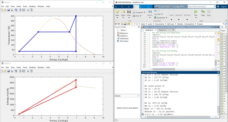
Step 5: Figure command is used to generate the plot with xlabel and ylabel to provide labels to the graphical representation of x-axis and y-axis. First figure is for plotting the temperature and entropy and second figure is for plotting entropy and enthalpy.

Main Code:

%cleaning
clear all
close all
clc

%displaying the process in different stages
fprintf('RANKINE CYCLE SIMULATOR\n')
fprintf('1-2 is Isentropic Expansion in the Turbine \n')
fprintf('2-3 is Constant Pressure heat Rejection by the Condensor \n')
fprintf('3-4 is Isentropic Compression in the Pump \n')
fprintf('4-1 is Constant Pressure Heat Addition by the Boiler \n')

%To enter the input for state point calculation
P1=input('Enter the Pressure at the Turbine Inlet (in bar):')
T1=input('Enter the Temperature at the Turbine inlet (in Degree Celcius:')
P2=input('Enter the Pressure at the Condenser (in bar):')

%to calculate te state point values - State point 1
H1=XSteam('h_pT',P1,T1) %Enthalpy at state point 1
S1=XSteam('s_pT',P1,T1) %Entropy at state point 1

%to calculate te state point values - State point 2&3
S2=S1;
P3=P2; %constant pressure heat rejection in condenser
s_f2=XSteam('sL_p',P2);
s_g2=XSteam('sV_p',P2);
h_f2=XSteam('hL_p',P2);
h_g2=XSteam('hV_p',P2);
S3=XSteam('sL_p',P3);
H3=XSteam('hL_p',P3);
T2=XSteam('Tsat_p',P3)
T3=T2;
H2=h_g2;

%to calculate te state point values - State point 4
S4=S3;%Isentropic compression
P4=P1;%constant pressure 
T4=XSteam('T_ps',P4,S4);
H4=XSteam('h_pT',P4,T4);
H4_1=XSteam('hL_p',P4);
S4_1=XSteam('sL_p',P4);
H4_2=XSteam('sV_p',P4);
S4_2=XSteam('sV_p',P4);
T4_1=XSteam('T_hs',H4_1,S4_1);
T4_2=XSteam('T_hs',H4_2,S4_2);

%work done in turbine
Wt=H1-H2;
%Work done in pump
Wp=H4-H3;
%net work done
Wnet=Wt-Wp;
%thermal efficiency
Q1=H1-H4;%Heat addition to the system
Q2=H2-H3 %Heat rejection from the system
Ntherm=((Wt-Wp)/Q1)*100;
%Specific Steam consumption
SSC=(3600/Wnet);

%Calculating T,S,and H at the vapour and liquid 
T6=XSteam('Tsat_p',P1);
S5=XSteam('sL_p',P1);
S6=XSteam('sV_p',P1);
H5=XSteam('hL_p',P1);
H6=XSteam('hV_p',P1);
T5=T6;

%Printing the output to command window
fprintf('\n RESULTS \n')
fprintf('At state point 1: \nP1 is : %4.2f \nT1 is : %4.2f Degree Celcius \nH1 is : %4.2f kJ/kg\nS1 is : %4.2f kJ/kgK\n\n', P1,T1,H1,S1)
fprintf('At state point 2: \nP2 is : %4.2f \nT2 is : %4.2f Degree Celcius \nH2 is : %4.2f kJ/kg\nS2 is : %4.2f kJ/kgK\n\n', P2,T2,H2,S2)
fprintf('At state point 3: \nP3 is : %4.2f \nT3 is : %4.2f Degree Celcius \nH3 is : %4.2f kJ/kg\nS3 is : %4.2f kJ/kgK\n\n', P3,T3,H3,S3)
fprintf('At state point 4: \nP4 is : %4.2f \nT4 is : %4.2f Degree Celcius \nH4 is : %4.2f kJ/kg\nS4 is : %4.2f kJ/kgK\n\n', P4,T4,H4,S4)
fprintf('Wt is :%4.2f kJ/Kg\nWp is : %4.2f kJ/Kg\nWnet is : %4.2f kJ/Kg\nNtherm is : %4.2f percent\nS.S.C is : %4.2f kg/kWh',Wt,Wp,Wnet,Ntherm,SSC)

temperature_ranges=linspace(0,550,1000);
for i=1:length(temperature_ranges)
    s_v(i)=XSteam('sV_T',temperature_ranges(i));
    s_l(i)=XSteam('sL_T',temperature_ranges(i));
    h_v(i)=XSteam('hV_T',temperature_ranges(i));
    h_l(i)=XSteam('hL_T',temperature_ranges(i));
end

%To plot Entropy and temperature
figure(1)
plot([S1 S2],[T1 T2],[S2 S3],[T2 T3],[S3 S4],[T3 T4],[S5 S6],[T5 T6],[S6 S1],[T6 T1],[S4 S4_1],[T4 T4_1],[S4_1 S4_2],[T4_1 T4_2],[S4_2 S4_1],[T4_2 T4_1],'marker','o','color','b','LineWidth',2)
hold on
plot(s_v,temperature_ranges)
plot(s_l,temperature_ranges)
xlabel('Entropy S [kJ/KgK] '); %x axis label
ylabel('Temperatures T [K] '); %y axis label
title('Temperature(T) - Entropy(S) Plot') %title for the plot

%To plot Entropy and Enthalpy
figure(2)
plot([S1 S2],[H1 H2],[S2 S3],[H2 H3],[S3 S4],[H3 H4],[S4 S1],[H4 H1],'marker','o','color','r','LineWidth',2)
hold on
plot(s_v,h_v)
plot(s_l,h_l)
xlabel('Entropy S [kJ/KgK] '); %X aixs label
ylabel('Enthalpy H [kJ/K] '); %y axis label
title('Enthalpy(H) - Entropy(S) Plot') %title for the plot

Inputs entered in command window:

Results Output:

All the state variable at different stages from 1,2,3 and 4 were determined and executed as follows:

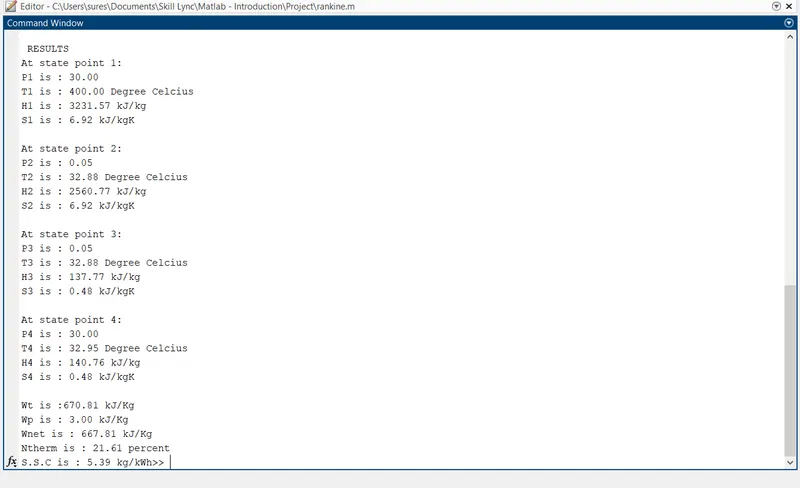
Net work output is: 667.01 kJ/Kg

Plot Output:

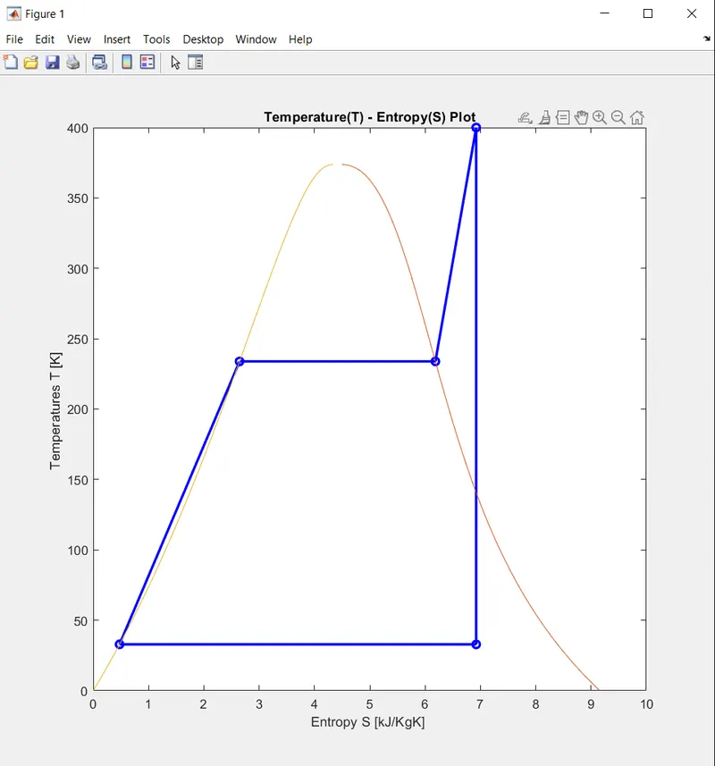
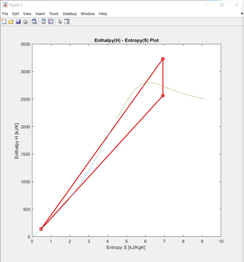
The T-S and S-H were plotted for the rankine cycle using the Xsteam data file provided where there is a process of isobaric heat transfer or constant pressure heat addition in a boiler, Isentropic expansion or isentropic expansion in the turbine, Isobaric Heat rejection or constant pressure heat rejection in a condenser and Isentropic compression or otherwise known as Isentropic compression in a pump.

Errors:

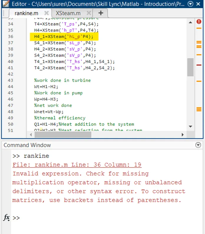
Error 1: Typo error: I forgot to include , in between 'hL_p and P4 as highlighted below.

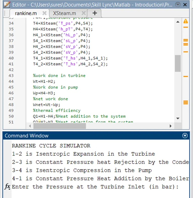
Rectified Solution: The above error was further rectified by including the , in between the variables.

Error 2: Typo Error: Included wrong representation of variable S_l instead of s_l

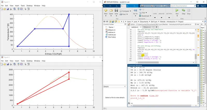
Rectified Solution: Rectified the program by changing the capital S to small letter s_l.

References:

Rankine cycle

https://mechanicalboost.com/rankine-cycle/

Theory Rankine

https://www.nuclear-power.com/nuclear-engineering/thermodynamics/thermodynamic-cycles/rankine-cycle-steam-turbine-cycle/theory-of-rankine-cycle-equations-and-calculation/#:~:text=During%20a%20Rankine%20cycle%2C%20the,and%204%20(isentropic%20expansion).