Project 2 - Rankine cycle Simulator

Aim:

To understand the concept of Rankine cycle by referring to standard thermal engineering text book.

To create a Rankine Cycle Simulator using OCTAVE/MATLAB.

To calculate the state points of the Rankine Cycle based on inputs specification.

To plot the corresponding T-s and h-s plots for the given set of inputs.

Inputs given:

Turbine Inlet temperature = 400° C

Turbine Inlet Pressure = 30 bars

Turbine Outlet Pressure = 0.05 bars = Condenser Inlet Pressure

To Calculate the followings,

• Net work output
• Back work ratio

Hints:

1.Code the basic program that calculates the state points alone

2.Then add the thermodynamic relation to get the points inbetween the state variables.

Program code:

clear all
close all
clc

fprintf('SIMULATOR Of RANKINE CYCLE \n')
fprintf('1-2 Isentropic expansion in the turbine \n')
fprintf('2-3 constant pressure heat rejection by the condensor \n')
fprintf('3-4 isentropic compression in the pump \n')
fprintf('4-1 constant pressure heat addition by the boiler \n')

%inputs
p1=input('enter the pressure at the turbine inlet(in bar):');
t1=input('enter the temperature at the turbine inlet(in degree celsius):');
p2=input('enter the pressure at the condensor(in bar):');
disp('results')
%getting cp & cv values from xsteam
%for vapour
high_cpV=XSteam('CpV_p',p1);
low_cpV=XSteam('CpV_p',p2);
high_cvV=XSteam('CvV_p',p1);
low_cvV=XSteam('CvV_p',p2);
%for liquid
high_cpL=XSteam('cpL_p',p1);
low_cpL=XSteam('cpL_p',p2);
high_cvL=XSteam('cvL_p',p1);
low_cvL=XSteam('cvL_p',p2);

%getting important parameters from xsteam
%for high pressure
t1s=XSteam('tsat_p',p1);
s1g=XSteam('sV_p',p1);
s1f=XSteam('sL_p',p1);
s1fg=s1g-s1f;
h1f=XSteam('hL_p',p1);
h1g=XSteam('hV_p',p1);
h1fg=h1g-h1f;
%for low pressure
s2g=XSteam('sV_p',p2);
s2f=XSteam('sL_p',p2);
s2fg=s2g-s2f;
t2s=XSteam('tsat_p',p2);
h2f=XSteam('hL_p',p2);
h2g=XSteam('hV_p',p2);
h2fg=h2g-h2f;

%%state point 1
disp('at state point 1:')
fprintf('p1 is :%f bar \n',p1)
fprintf('t1 is :%f deg celsius',t1)
h1=XSteam('h_pt',p1,t1);
fprintf('h1 is :%f kJ/kg \n',h1)
s1=XSteam('s_pt',p1,t1);
fprintf('s1 is :%f kJ/kg \n',s1)

%%state point 2
disp('at state point 2:')
fprintf('p2 is :%f bar \n',p2)
s2=s1,
fprintf('s2 is :%f kJ/kgk \n',s2)
%predicting location of point 2 in T-S
if(s2<=s2g)
    x2=(s2-s2f)/(s2fg);
else
    x2=1;
end
fprintf('x2 is :%f \n',x2)
%calculating t2
if(x2<1)
    t2=t2s;
else
    %t2 calculate by s2=s2g+low_cpV*(log(t2/t2s))
    t2=(t2s+273.15)*exp((s2-s2g)/low_cpV);
    t2=t2-273.15;
end
fprintf('t2 is : %f deg celsius \n',t2)
if(x2<1)
    h2=h2f+x2*h2fg;
else
    h2=h2g+low_cpV*(t2-t2s);
end
fprintf('h2 is : %f kJ/kg \n',h2)

%%state point 3
%assuming no subcooling in condensor
disp('at state point 3:')
p3=p2;
fprintf('p3 is : %f bar \n',p3)
v3=XSteam('vL_p',p3);
t3=t2s;
fprintf('t3 is : %f deg celsius \n', t3)
h3=h2f;
fprintf('h3 is : %f kJ/kg \n', h3)
s3=s2f;
fprintf('s3 is : %f kJ/kg \n', s3)

%%state point 4
disp('at state point 4:')
p4=p1;
fprintf('p4 is : %f bar \n',p4)
s4=s3;
fprintf('s4 is : %f kJ/kgk \n', s4)
wp=v3*(p4-p3)*100;
h4=wp+h3;
fprintf('h4 is : %f kJ/kg \n', h4)

%to calculate t4 s4=s3=sf1-high_cpL*ln/t1s?t4
term=exp((s1f-s4)/high_cpL);

t4=t1s/term;
fprintf('t4 is : %f deg celsius \n',t4)

%%work done,heat,ssc & efficiency calculation
wt=h1-h2;
fprintf('work done by turbine is : %f kJ/kg \n', wt)
fprintf('work done by compressor is : %f kJ/kg \n', wp)
wnet=wt-wp;
fprintf('net work done is : %f kJ/kg \n', wnet)
qin=h1-h4;
eff_thermal=wnet/qin;
fprintf('thermal efficiency is : %f ',eff_thermal);
ssc=3600/wt;
fprintf('s.s.c is : %f kg/kwh', ssc)

%%calculating for plotting liquid & vapout lies
%
%<>
%
temperature=linspace(1,373,500);
for i=1:length(temperature)
    h_L(i)=XSteam('hL_t',temperature(i));
    h_V(i)=XSteam('hV_t',temperature(i));
    s_L(i)=XSteam('sL_t',temperature(i));
    s_V(i)=XSteam('sV_t',temperature(i));
end

%%plotting T-S & H-S diagram
figure(1) % T-S
hold on
plot([s1 s2],[t1 t2],'r','linewidth',1)
text(s1,t1,'1')
text(s2,t2,'2')
plot([s2 s2g],[t2 t2s],'r','linewidth',1)
text(s2g,t2s,'2s')
plot([s2g s3],[t2s t3],'r','linewidth',1)
text(s3,t3,'3')
plot([s3 s4],[t3 t4],'r','linewidth',1)
text(s4,t4,'4')
plot([s4 s1f],[t4 t1s],'r','linewidth',1)
text(s1f,t1s,'4s')
plot([s1f s1g],[t1s t1s],'r','linewidth',1)
text(s1g,t1s,'1s')
plot([s1g s1],[t1s t1],'r','linewidth',1)
plot(s_L,temperature,'b','linestyle','--','linewidth',1)
plot(s_V,temperature,'b','linestyle','--','linewidth',1)
%marking direction
text(s1,(t1+t2)/2,'\vee','color','r')
text((s2g+s2f)/2,t3,'\angle','color','r')
text(s3,(t3+t4)/2,'\wedge','color','r')
text((s1f+s1g)/2,t1s,'\angle','color','r')
title('T-S diagram of Ideal Rankine cycle')
xlabel('specific entropy(kJ/kgk)')
ylabel('temperature(deg c)')

figure(2)%h-s
hold on
plot([s1 s2],[h1 h2],'r','linewidth',1);
text(s1,h1,'1')
plot([s2 s3],[h2 h3],'r','linewidth',1);
text(s2,h2,'2')
plot([s3 s4],[h3 h4],'r','linewidth',1);
text(s3,h3,'3')
plot([s4 s1],[h4 h1],'r','linewidth',1);
text(s4,h4,'4')
plot(s_L,h_L,'b','linestyle','--','linewidth',1.5)
plot(s_V,h_V,'b','linestyle','--','linewidth',1.5)
title('h-s diagram','fontsize',15)
xlabel('specific entropy(kJ/kgk)')
ylabel('specific enthalpy(kJ/kg)')

Explanation:

Downloaded the XSteam file and saved to the same folder where the program for Rankine is done.

Now the initiation to the program by defining and declaring all the functions involved in the Rankine cycle is carried out.

Major inputs are pressure,temperature and volume at the inlet and exit,which are categorized as follows,

1-2: Isentropic expansion in the turbine

2-3:Constant pressure heat rejection by the condenser

3-4:Isentropic compression in the pump

4-1:Constant pressure heat addition by the boiler

Units are considered as bar for pressure, deg C for temperature and refernces are made for all the other parameters from the XSteam table.

The working medium of fluid is water and the process whenit undergoes, coverts into vapour, so those two states are considered.

The specific enthalpy specific entropy and temperature functions are declared to obtain the plot for the same rankine cycle process.

For liquid and for vapour, the steam functions are declared followed by which the important parameters for high temperature and for the low temperature are defined.

Then the state varibles for 1,2,3,4 are declared as per the given statement.

After declaring the state variables,work done,efficiency calcualtion are carried out using appropriate relations.

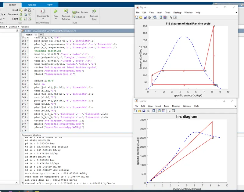
Finally plots for the same are carried out, T-S and h-s diagram which shows the temperature entropy relation and enthalpy vs entropy relation.

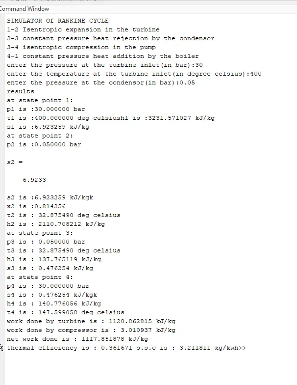
Screenshot:

Result:

The concept of Rankine cycle by referring to standard thermal engineering text book was done.

Created a Rankine Cycle Simulator using OCTAVE/MATLAB.

Calculated the state points of the Rankine Cycle based on inputs specification.

Plotted the corresponding T-s and h-s plots for the given set of inputs.