Project 2 - Rankine cycle Simulator

Objectives :

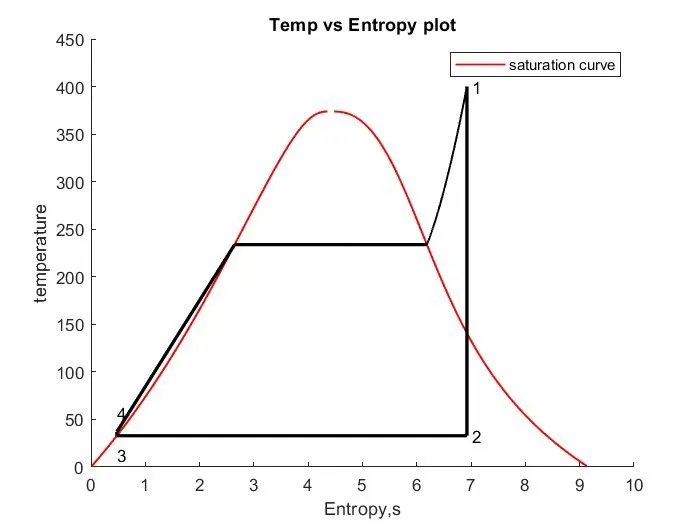
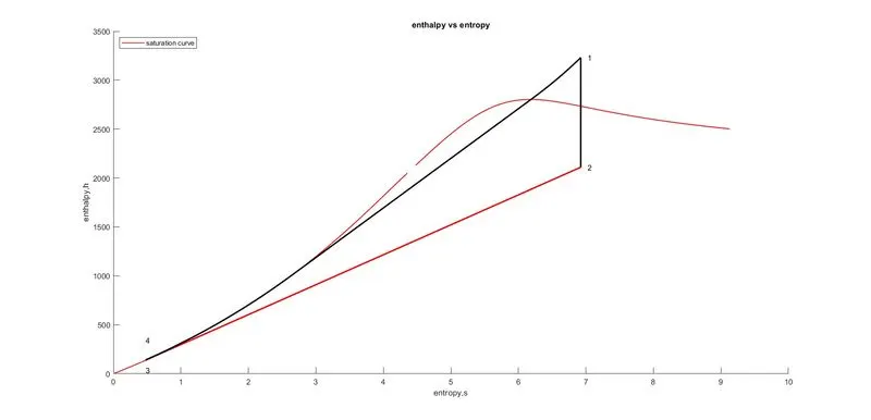
To write a program to stimulate the rankine cycle by calculating and plotting the points corresponding to the state points and joining the gap between them and identify them as process on both T-s and H-s plots with the net work and back power ratio.

Introduction :

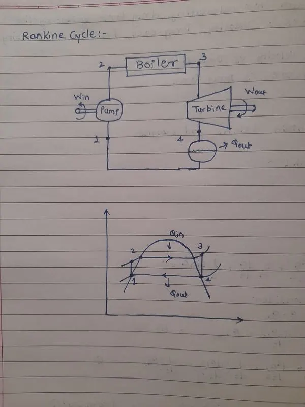
Rankine cycle is a vapour power cycle it is much more practical than the carnot cycle with good efficiency rates is is also has a scope to improve the efficiency by a lot of methods such as regeneration and reheating. this makes the rankine cycle on ideal cycle for the steam turbines.

Working :

1-2 isentropic compression process

after going through the condenser , the water gets into liquid state, in this process the pump transfers, the water towards the boiler , the pump increases the pressure , compression and leaves its boiler.

2-3 isobaric heat addition process

The high-pressure liquid enters a boiler , where it is heated at constant pressure by an external heat source to become a dry saturated vapour. inlet of the turbines needs to be fed with water at high pressure and teperature

3-4 isentropic expansion process

the hot steam coming out from the bpoler is fed to the turbines. the superheated water hits blade of the turbines at high temperature and pressure. in rotation if the turbine blade and as a results , waer losses its temperature and pressure.

4-1 isobaric heat rejection process

output leftover from the turbines from a boiler fed into the codenser. To reuse the water again, it has to be brought back to the saturated liquid state. the condenser absorbs heat from the water and brings its to saturated water state at constant oressure

worked is obtained from the turbine and work is consumed from pump, along with this, hear is supplied at the boiler and rejected at the condenser.

by repeating above cycle

Equations :

• Wnet = Wt-Wp
• efficiency = (Wnet/Qs)X10 - Q is net heat supplied.
• back power ratio = Wp/Wt
• Wp and Wt are the work done by turbine and pump repectively.
• Wr + BWR = 1
• Heat rate = 1/ effeciency
• steam rate (SSC ) = 1/ (wnet)

Code :

clear all

close all

clc

%program for rankin cycle simulation

%1=turbine inlet

%2= turbine oulet

%3=pump inlet

%4=pump outlet

%input parameters

%p1= turbine inlet pressure

%t1=turbine inlet temperature

%p2=Turbine outlet pressure

% Description of the process

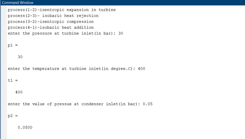
disp('process(1-2)-isentropic expansion in turbine')

disp('process(2-3)- isobaric heat rejection')

disp('process(3-2)-isentropic compression')

disp('process(4-1)-isobaric heat addition')

%for state variable input at point 1

p1=input('enter the pressure at turbine inlet(in bar): ')

t1=input('enter the temperature at turbine inlet(in degree.C): ')

p2=input('enter the value of pressue at condenser inlet(in bar): ')

%extrating data

%state 1

h1=XSteam('h_pT',p1,t1);

s1=XSteam('s_pT',p1,t1);

%state 2

s2=s1;

sf2=XSteam('sL_p',p2);

sg2=XSteam('sV_p',p2);

x2=(s2-sf2)/(sg2-sf2);

hf2=XSteam('hL_p',p2);

hg2=XSteam('hV_p',p2);

h2=hf2+(x2*(hg2-hf2));

%state 3

p3=p2

s3=XSteam('sL_p',p3);

h3=XSteam('hL_p',p3');

%state 4

s4=s3;

p4=p1

%work done by turbine

wt=h1-h2;

%work done to run pump

v3=XSteam('vL_p',p3);

wp=v3*(p4-p3)*100;

h4=h3+wp;

%net work

wnet=wt-wp;

%heat into system

qin=h1-h4;

%heat out of system

qout=h2-h3;

%thermal efficiency

eff=(wnet/qin)*100;

%specific steam consumption

%ssc=mass flow rate/power;

ssc=(3600/wnet);

%calculating temperature at state points

t3=XSteam('Tsat_p',p3);

t2=t3;

cp4=XSteam('Cp_ps',p4,s4);

cv4=XSteam('Cv_ps',p4,s4);

k=cp4/cv4;

t4=t3/((p3/p4)^((k-1)/k));

% back work ratio

back_work_ratio=(wp/wt);

%line for plotting

t6=XSteam('Tsat_p',p1);

s5=XSteam('sL_p',p1);

s6=XSteam('sV_p',p1);

h5=XSteam('hL_p',p1);

h6=XSteam('hV_p',p1);

t5=t6;

%plotting the saturation curve

T=linspace(1,375,1000);

for i=1:length(T)

sf(i)=XSteam('sL_T',T(i));

sg(i)=XSteam('sV_T',T(i));

hf(i)=XSteam('hL_T',T(i));

hg(i)=XSteam('hV_T',T(i));

end

%plotting T-S diagram

figure(1)

hold on

plot(sf,T,'r','linewidth',1)

plot(sg,T,'r','linewidth',1)

plot([s1 s2],[t1 t2],'k','linewidth',2)

plot([s2 s3],[t2 t3],'k','linewidth',2)

plot([s3 s4],[t3 t4],'k','linewidth',2)

plot([s4 s5],[t4 t5],'k','linewidth',2)

plot([s5 s6],[t5 t6],'k','linewidth',2)

sc1=linspace(s6,s1,1000);

for l=1:length(sc1)

Tc1(l)=XSteam('T_ps',p1,sc1(l));

end

plot(sc1,Tc1,'k','linewidth',1)

text(s1+0.1,t1,'1')

text(s2+0.1,t2,'2')

text(s3,t3-20,'3')

text(s4,t4+20,'4')

title('Temp vs Entropy plot')

xlabel('Entropy,s')

ylabel('temperature')

legend('saturation curve')

%plot h-s diagram

figure(2)

hold on

plot(sf,hf,'r','linewidth',1)

plot(sg,hg,'r','linewidth',1)

plot([s1 s2],[h1 h2],'k','linewidth',2)

plot([s2 s3],[h2 h3],'r','linewidth',2)

plot([s3 s4],[h3 h4],'r','linewidth',2)

hc=linspace(h4,h5,100);

for k=1:length(hc)

sch(k)=XSteam('s_ph',p1,hc(k));

end

plot(sch,hc,'k','lineWidth',2 )

plot([s5 s6],[h5 h6],'k','linewidth',2)

for m=1:length(sc1)

hc1(m)=XSteam('h_ps',p1,sc1(m));

end

plot(sc1,hc1,'k','linewidth',2)

text(s1+0.1,h1,'1')

text(s2+0.1,h2,'2')

text(s3,h3-100,'3')

text(s4,h4+200,'4')

title('enthalpy vs entropy')

xlabel('entropy,s')

ylabel('enthalpy,h')

legend('saturation curve','location','northwest')

%Display results

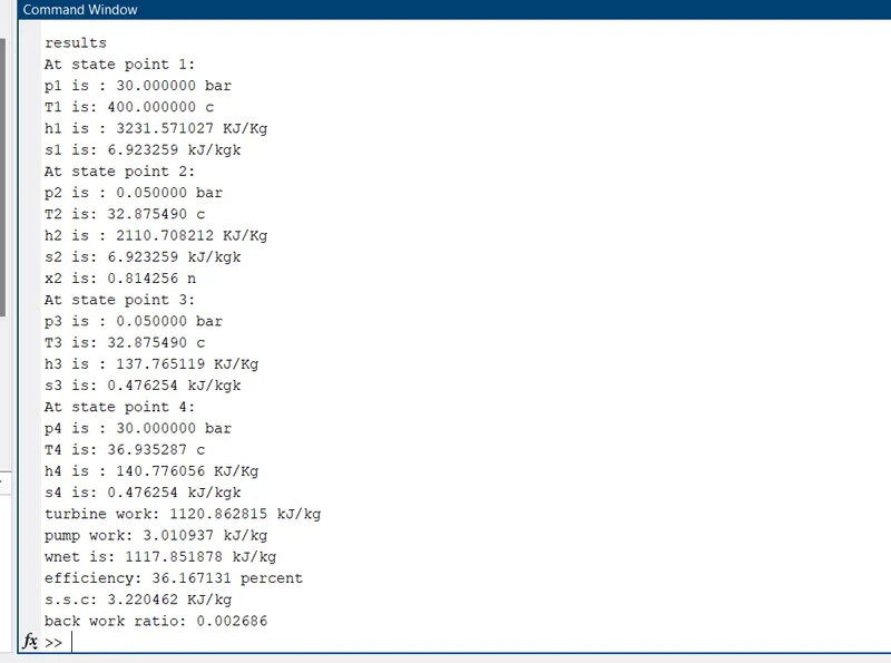
disp('results')

fprintf('At state point 1: \n');

fprintf('p1 is : %f bar \n',p1);

fprintf('T1 is: %f c \n',t1);

fprintf('h1 is : %f KJ/Kg \n',h1);

fprintf('s1 is: %f kJ/kgk \n',s1);

fprintf('At state point 2: \n');

fprintf('p2 is : %f bar \n',p2);

fprintf('T2 is: %f c \n',t2);

fprintf('h2 is : %f KJ/Kg \n',h2);

fprintf('s2 is: %f kJ/kgk \n',s2);

fprintf('x2 is: %f n \n',x2);

fprintf('At state point 3: \n');

fprintf('p3 is : %f bar \n',p3);

fprintf('T3 is: %f c \n',t3);

fprintf('h3 is : %f KJ/Kg \n',h3);

fprintf('s3 is: %f kJ/kgk \n',s3);

fprintf('At state point 4: \n');

fprintf('p4 is : %f bar \n',p4);

fprintf('T4 is: %f c \n',t4);

fprintf('h4 is : %f KJ/Kg \n',h4);

fprintf('s4 is: %f kJ/kgk \n',s4);

fprintf('turbine work: %f kJ/kg \n',wt);

fprintf('pump work: %f kJ/kg \n',wp);

fprintf('wnet is: %f kJ/kg \n',wnet);

fprintf('efficiency: %f percent \n',eff);

fprintf('s.s.c: %f KJ/kg \n',ssc);

fprintf('back work ratio: %f \n',back_work_ratio);

Code Input :

Results :

Graphs :

Explanation :

• To stimulate and found different state variables, all the process parameters are to be described such as all four process ocuring and input parameters.
• standard Xsteam library to get table data for water , all points in between state variables are calculated.
• plot propery diagram of water , T-s & H-s diagram and marked using command.