Project 2 - Rankine cycle Simulator

• Aim :-Create a Rankin Cycle Simulator using OCTAVE/MATLAB.
• Objective :-

• To calculate the state points of the rankine cycle based on user input.
• To plot the corresponding T-s and h-s plots for the given set of inputs.

• Theory

• Basic Cycle
• The Rankine cycle is the fundamental operating cycle of all power plants where an operating fluid is continuously evaporated and condensed. The selection of operating fluid depends mainly on the available temperature range. Figure 1 shows the idealized Rankine cycle.
• The pressure-enthalpy (p-h) and temperature-entropy (T-s) diagrams of this cycle are given in Figure 2. The Rankine cycle operates in the following steps:
• 1-2-3 Isobaric Heat Transfer. High pressure liquid enters the boiler from the feed pump (1) and is heated to the saturation temperature (2). Further addition of energy causes evaporation of the liquid until it is fully converted to saturated steam (3).
• 3-4 Isentropic Expansion. The vapor is expanded in the turbine, thus producing work which may be converted to electricity. In practice, the expansion is limited by the temperature of the cooling medium and by the erosion of the turbine blades by liquid entrainment in the vapor stream as the process moves further into the two-phase region. Exit vapor qualities should be greater than 90%.
• 4-5 Isobaric Heat Rejection. The vapor-liquid mixture leaving the turbine (4) is condensed at low pressure, usually in a surface condenser using cooling water. In well designed and maintained condensers, the pressure of the vapor is well below atmospheric pressure, approaching the saturation pressure of the operating fluid at the cooling water temperature.
• 5-1 Isentropic Compression. The pressure of the condensate is raised in the feed pump. Because of the low specific volume of liquids, the pump work is relatively small and often neglected in thermodynamic calculations.

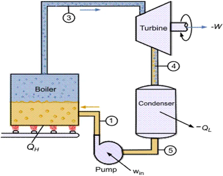
• Figure 1. Rankine cycle.

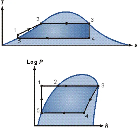
• Figure 2. T-s and p-h diagrams.

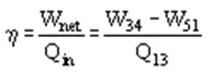
• The efficiency of power cycles is defined as
• 
• Values of heat and work can be determined by applying the First Law of Thermodynamics to each step. The steam quality x at the turbine outlet is determined from the assumption of isentropic expansion, i.e.,
• 
• where is the entropy of vapor and Si* the entropy of liquid.

Technical terms :-

Enthalpy :- the sum of the internal energy and the product of the pressure and volume of a thermodynamic system.

Entropy :- the measure of a system’s thermal energy per unit temperature that is unavailable for doing useful work. Because work is obtained from ordered molecular motion, the amount of entropy is also a measure of the molecular disorder, or randomness, of a system.

Formulae :-

Applying steady flow energy equation (S.F.E.E.) to boiler, turbine, condenser and pump :

(i) For boiler (as control volume),

we get

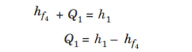
(ii) For turbine (as control volume), we get

(iii) For condenser, we get

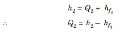
(iv) For the feed pump, we get

Now, efficiency of Rankine cycle is given by

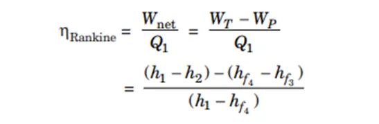
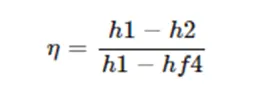
When hf4 – hf3 value is very small then

IMPORTANT TERMS RELATING STEAM FORMATION

1. Sensible heat of water (hf ). It is defined as the quantity of heat absorbed by 1 kg of water when it is heated from 0°C (freezing point) to boiling point. It is also called total heat (or enthalpy) of water or liquid heat invariably. It is reckoned from 0°C where sensible heat is taken as zero. If 1 kg of water is heated from 0°C to 100°C the sensible heat added to it will be 4.18 × 100 = 418 kJ but if water is at say 20°C initially then sensible heat added will be 4.18 × (100 – 20) = 334.4 kJ. This type of heat is denoted by letter hf and its value can be directly read from the steam tables.

Note. The value of specific heat of water may be taken as 4.18 kJ/kg K at low pressures but at high pressures it is different from this value.

2. Latent heat or hidden heat (hfg). It is the amount of heat required to convert water at a given temperature and pressure into steam at the same temperature and pressure. It is expressed by the symbol hfg and its value is available from steam tables. The value of latent heat is not constant and varies according to pressure variation.

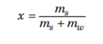
3. Dryness fraction (x). The term dryness fraction is related with wet steam. It is defined as the ratio of the mass of actual dry steam to the mass of steam containing it. It is usually expressed by the symbol ‘x’ or ‘q’.

If ms = Mass of dry steam contained in steam considered, and

mw = Weight of water particles in the steam considered,

Then,

4. Total heat or enthalpy of wet steam (h). It is defined as the quantity of heat required to convert 1 kg of water at 0°C into wet steam at constant pressure. It is the sum of total heat of water and the latent heat and this sum is also called enthalpy.

In other words, h = hf + xhfg

If steam is dry and saturated, then x = 1 and hg = hf + xhfg

5. Superheated steam. When steam is heated after it has become dry and saturated, it is called superheated steam and the process of heating is called superheating. Superheating is always carried out at constant pressure. The additional amount of heat supplied to the steam during superheating is called as ‘Heat of superheat’ and can be calculated by using the specific heat of superheated steam at constant pressure (cps), the value of which varies from 2.0 to 2.1 kJ/ kg K depending upon pressure and temperature.

If Tsup., Ts are the temperatures of superheated steam in K and wet or dry steam, then

(Tsup – Ts) is called ‘degree of superheat’.

The total heat of superheated steam is given by

hsup = hf + hfg + cps (Tsup – Ts )

6. Volume of wet and dry steam. If the steam has dryness fraction of x, then 1 kg of this steam will contain x kg of dry steam and (1 – x) kg of water. If vf is the volume of 1 kg of water and vg is the volume of 1 kg of perfect dry steam (also known as specific volume), then volume of 1 kg of wet steam = volume of dry steam + volume of water.

= xvg + (1 – x)vf

Note. The volume of vf at low pressures is very small and is generally neglected. Thus is general, the

volume of 1 kg of wet steam is given by, xvg and density 1 xvg kg/m3 .

= xvg + vf – xvf

= vf + x(vg – vf )

= vf + xvfg

= vf + xvfg + vfg – vfg

= (vf + vfg) – (1 – x) vfg

= vg – (1 – x)vfg

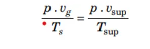
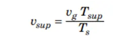
7. Volume of superheated steam. As superheated steam behaves like a perfect gas its volume can be found out in the same way as the gases.

If, vg = Specific volume of dry steam at pressure p,

Ts = Saturation temperature in K

Tsup = Temperature of superheated steam in K, and

vsup = Volume of 1 kg of superheated steam at pressure p,

Or

Steam condition :-

Based on the nature of the steam in the turbine inlet, the three types of condition is proposed. The three conditions are,

• Wet steam (x<1)
• Saturated steam (x=1)
• Super saturated steam (x>1)

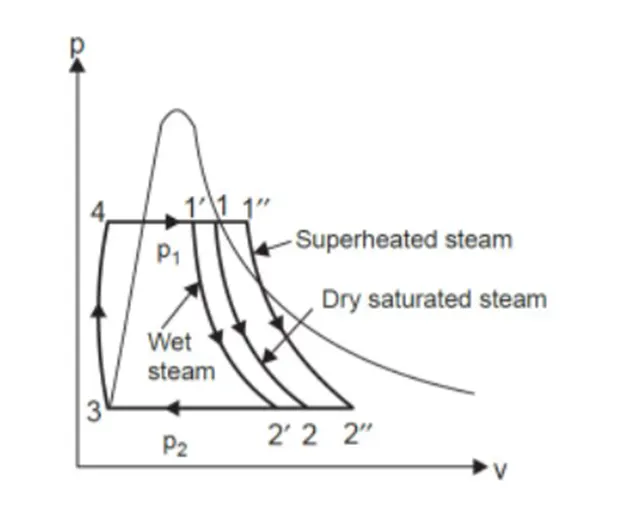
The ‘x’ value is defined as the dryness fraction based on the dryness fraction value the conditions can be classified. The ‘x’ value can be calculated by using the formula given below,

Hi = hfi + x(hfgi) where I is the position in which all datas are known.

Main Code -

clear all
close all
clc

% Simulating Rankine Cycle
% Process Description
fprintf('1-2 Isobaric heat Transfer\n')
fprintf('2-3 Isentropic Expansion\n')
fprintf('3-4 Isobaric heat rejection\n')
fprintf('4-1 Isentropic compression\n')

% Inputs
p1 = input('Enter the pressure at the turbine inlet(in bar)');
t1 = input('Enter the Temperature at the inlet(in Degree Celcius)');
p2 = input('Enter the pressure at condenser(in bar)');

%Input conditions
t = XSteam('Tsat_p',p1);
if t1>=t
h1 = XSteam('h_pT',p1,t1);
s1 = XSteam('s_pT',p1,t1);
end
%State points Evaluation
p4 = p1;
p3 = p2;
h3 = XSteam('hL_p',p3);
s3 = XSteam('sL_p',p3);
t3 = XSteam('Tsat_p',p3);
s2 = s1;
t2 = t3;
sf2 = XSteam('sL_p',p2);
sg2 = XSteam('sV_p',p2);
x2 = (s2 - sf2)/(sg2 - sf2);
hf2 = XSteam('hL_p',p2);
hg2 = XSteam('hV_p',p2);
h2 = hf2 + x2*(hg2 - hf2);
s4 = s3;
h4 = XSteam('h_ps',p4,s4);
cp4 = XSteam('Cp_ps',p4,s4);
cv4 = XSteam('Cv_ps',p4,s4);
g4 = cp4/cv4; 
o = (g4 - 1)/g4;
t4 = t3*((p4/p3)^o);

% Turbine & Pump Work
wt = h1 - h2;
wp = h4 - h3;

% net work
wnet = wt - wp;

% heat supplied
qs = h1 - h4;

% Efficiency
n_per = (wnet/qs)*100;

%Steam rate per second
stm_rate = 3600/(wt - wp);

% For process 4-1, which is isobaric we use the expression dH = Cp*dT
t5 = XSteam('Tsat_p',p1);
s5 = XSteam('sL_p',p1);
s6 = XSteam('sV_p',p1);

% output
fprintf('\n\tRESULT\n')
fprintf('At state point 1:\np1 is :%4.2 Bar\nT1 is :%4.2f Degree celcius\nH1 is :%4.2f KJ/Kg \nS1 is :%4.2f KJ/Kgk\n\n',p1,t1,h1,s1)
fprintf('At state point 2:\np2 is :%4.2 Bar\nT2 is :%4.2f Degree celcius\nH2 is :%4.2f KJ/Kg \nS2 is :%4.2f KJ/Kgk\n\n',p2,t2,h2,s2)
fprintf('At state point 3:\np3 is :%4.2 Bar\nT3 is :%4.2f Degree celcius\nH3 is :%4.2f KJ/Kg \nS3 is :%4.2f KJ/Kgk\n\n',p3,t3,h3,s3)
fprintf('At state point 4:\np4 is :%4.2 Bar\nT4 is :%4.2f Degree celcius\nH4 is :%4.2f KJ/Kg \nS4 is :%4.2f KJ/Kgk\n\n',p4,t4,h4,s4)
fprintf('Wt is :%4.2f KJ/Kg\nWp is :%4.2f KJ/Kg\nWnet is :%4.2f KJ/Kg\nNtherm is :%4.2f percent\nS.S.C is :%4.2f Kg/kWh',wt,wp,wnet,n_per,stm_rate)

% Vapour Line
temp = linspace(1,400,100);
for i = 1:length(temp)
    ent_l(i) = XSteam('sL_T',temp(i));
    ent_v(i) = XSteam('sV_T',temp(i));
    enth_l(i) = XSteam('hL_T',temp(i));
    enth_v(i) = XSteam('hV_T',temp(i));
end

% Plotting
subplot(1,2,1)
plot([s1 s2 s3 s4 s5 s6 s1],[t1 t2 t3 t4 t5 t5 t1],'color','k','linewidth',2,'markersize',2,'markerfacecolor','b','MarkerEdgeColor','b')
hold on
plot(ent_l,temp,'color','r')
plot(ent_v,temp,'color','r')
axis([0 10 0 700])
text(s1,t1,'1','FontSize',15)
text(s2,t2,'2','FontSize',15)
text(s3,t3,'3','FontSize',15,'HorizontalAlignment','left')
text(s4,t4,'4','FontSize',15,'HorizontalAlignment','right')
xlabel('Entropy')
ylabel('Temperature')
subplot(1,2,2)
plot([s1 s2 s3 s4 s1],[h1 h2 h3 h4 h1],'color','k','LineWidth',2,'marker','o','MarkerFaceColor','b','MarkerEdgeColor','b')
axis([0 10 300 5000])
hold on
plot(ent_v,enth_v,'color','r')
plot(ent_l,enth_l,'color','r')
text(s1,h1,'1','FontSize',15)
text(s2,h2,'2','FontSize',15)
text(s3,h3,'3','FontSize',15,'HorizontalAlignment','right','VerticalAlignment','top')
text(s4,h4,'4','FontSize',15,'HorizontalAlignment','right','VerticalAlignment','bottom')
xlabel('Entropy')
ylabel('Enthalpy')

Code Explanation :-

1. We will use standard XStream library to get the steam table data for water, is given below. It must be used to calculate the points in between the state variables.

2. Clearing workspace, command window and closing all plots

3. The user inputs that have to be entered by the usedr are:

Pressure at the turbine inlet (In bar)

Temperature at the turbine inlet (in Degree C)

Pressure at the condenser(in bar)

4. Based on the inputs we will calculate state variables by using equation of state and X_steam liabrary which is a stream table and we can directrly read values of state variables using it.

5.After calculating the state varuables at each state point we have calculated the turbine and pump work done.

6.At the end we plotted the corresponding T-s and h-s plots for the given set of inputs.

Abravitives Used -

Results :-

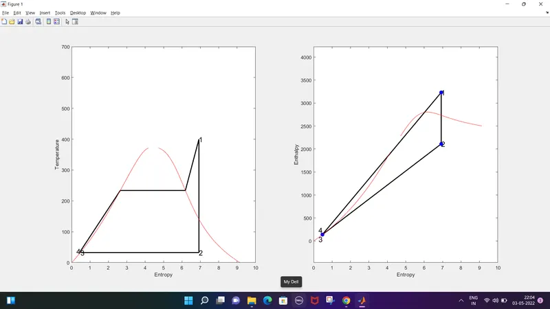
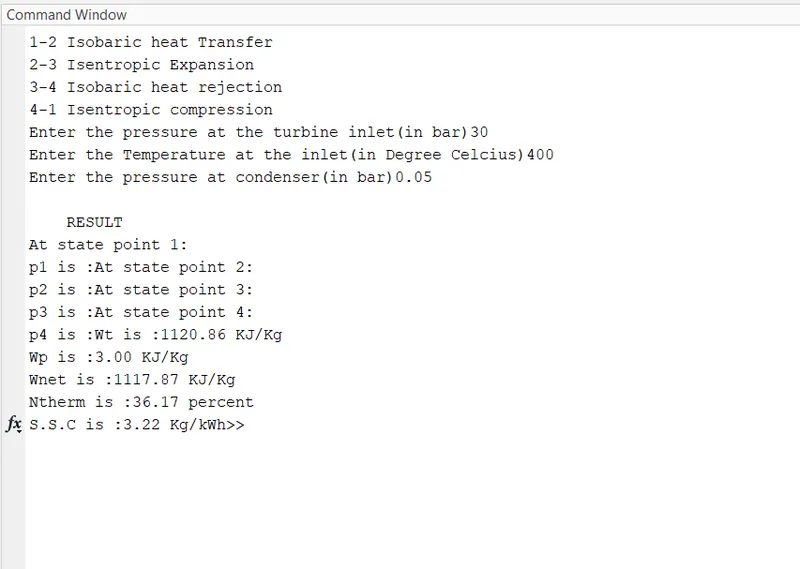
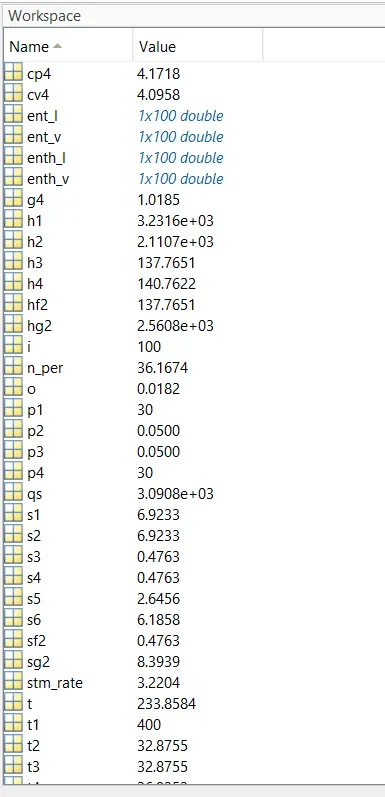
Calculate the followings,

• Net work output = 1117.87 KJ/Kg
• Back work ratio = 3.22 Kg/kWh.