Project 2 - Rankine cycle Simulator

• Aim : Create a Rankine Cycle Simulator using MATLAB .

• Objective :

1. Calculate the state points of the Rankine Cycle based on user inputs .
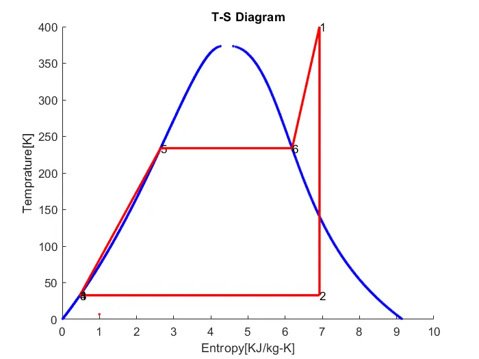
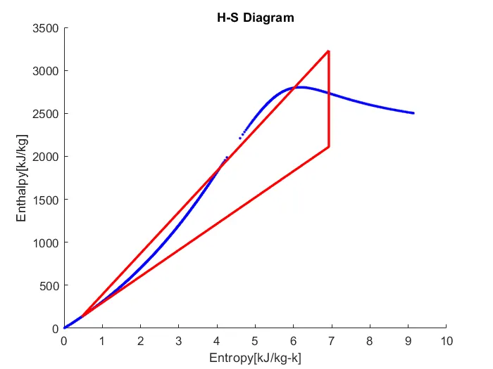
2. plot the corresponding T - s and h - s plots for the given set of inputs.

• Outputs :

1. Net work output
2. Back work ratio

• Given Inputs Value :

1. Turbine Inlet temperature = 400 ° C
2. Turbine Inlet Pressure = 30 bars
3. Turbine Outlet Pressure = 0.05 bars=Condenser Inlet Pressure

• Steam Table Data : - Standard XSteam library

• Rankine Cycle : -

• The Rankine cycle is an idealized thermodynamic cycle describing the process by which certain heat engines , such as steam turbines or reciprocating steam engines ,allow mechanical work to be extracted from a fluid as it moves between a heat source and heat sink .
• Heat energy is supplied to the system via a boiler where the working fluid ( typically water ) is converted to a high pressure gaseous state ( steam ) in order to turn a turbine .
• After passing over the turbine the fluid is allowed to condense back into a liquid state as waste heat energy is rejected before being returned to boiler , completing the cycle .
• Friction losses throughout the system are often neglected for the purpose of simplifying calculations as such losses are usually much less significant than thermodynamic losses , especially in larger systems.

• Four Processes in the Rankine Cycle:

• Process 1-2 : The working fluid is pumped from low to high pressure . As the fluid is a liquid at this stage , the pump requires little input energy .Process 1-2 is isentropic compression .

• Process 2-3 : The high - pressure liquid enters a boiler , where it is heated at constant pressure by an external heat source to become a dry saturated vapour . The input energy required can be easily calculated graphically , using an enthalpy - entropy chart ( h - s chart , or Mollier diagram ) , or numerically , using steam tables or software . Process 2-3 is constant pressure heat addition in boiler .

• Process 3-4 : The dry saturated vapour expands through a turbine , generating power . This decreases the temperature and pressure of the vapour , and some condensation may occur . The output in this process can be easily calculated using the chart or tables noted above . Process 3-4 is isentropic expansion .

• Process 4-1 : The wet vapour then enters a condenser , where it is condensed at a constant pressure to become a saturated liquid . Process 4-1 is constant pressure heat rejection in condenser.

STEP BY STEP CODE EXPLAINATION :

1.Described pressure and temperature values by user defined.

2.Find out the value of enthalpy ( h) and entropy ( s) from pressure and temperature from XSteam library in Matlab .

3.XSteam library is nothing but the steam table , which is put in the same directory where Matlab program saved

4. Find out all the points of inlet & outlet of turbine , condenser , pump and boiler.

5. Also find out the work done of pump and turbine.

6. Find out net work done , heat supplied , heat rejected , efficiency & specific steam consumption ,Back work ratio.

7. finally plot the H - S and T - S plots .

8. Link all the points of the cycle.

9. gives the , title , x-label & y-label .

10. Output the results values of P , T , H , S for each state respectively

clear all 
close all 
clc 

% Process Information 

fprintf('Rankine Cycle Simulator \n') 
fprintf('process 1-2:Isentropic Expansion \n') 
fprintf('process 2-3:Isobaric Heat Rejection \n') 
fprintf('process 3-4:Isentropic compression \n')
fprintf('process 4-1:Isobaric heat addition process \n')


% Initial Inputs
P1 = input('Enter the inlet pressure of Turbine:'); 
P2 = input('Enter the outlet pressure from Turbine:'); 
T1 = input('Enter the steam inlet Temperature:');


% State point 1 
H1 = XSteam('h_pT',P1,T1); % Enthalpy 
S1 = XSteam('s_pT',P1,T1); % Entropy 
Hf1= XSteam('hl_p',P1);    % Enthalpy of saturated liquid 
Hg1= XSteam('hV_p',P1);    % Enthalpy of saturated vapour 
Ts1= XSteam('Tsat_P',P1);  % Saturation Temp 
Sf1= XSteam('sL_p',P1);    % Entropy of saturated liquid 
Sg1= XSteam('sv_p',P1);    % Entropy of saturated vapour 


% State point 2 
S2 = S1;
Sf2 = XSteam('sL_p',P2);
Sg2 = XSteam('sV_p',P2); 
Hf2 = XSteam('hL_p',P2); 
Hg2 = XSteam('hV_p',P2);
x =(S2-Sf2)/(Sg2-Sf2);     % Dryness Fraction
H2 =Hf2+x*(Hg2-Hf2); 
T2 =XSteam('T_ph',P2,H2); 
Ts2=XSteam('Tsat_p',P2);


% State Point 3
H3 = Hf2 ; 
S3 = Sf2 ; 
T3 = T2 ; 
P3 = P2 ;


% State point 4 
P4 = P1 ; 
S4 = S3 ; 
H4 = XSteam('h_ps',P4,S4); 
T4 = XSteam('T_Ps',P4,S4); 


% State point 5
S5 = XSteam ('sL_p',P1);
H5 = XSteam('hL_p',P1);
T5 = XSteam('Tsat_p',P1);


% State point 6
S6 = XSteam ('sV_p',P1);
H6 = XSteam('hV_p',P1);
T6 = T5;

t = linspace(0,374,500); 

% Plot T-S Diagram 
figure(1) 
hold on 
for i = 1:length(t) 
    plot(XSteam('sL_T',t(i)),t(i),'.','color','b') 
    plot(XSteam('sV_T',t(i)),t(i),'.','color','b') 
end 


% Plot Cycle
plot([S1 S2],[T1 T2],'linewidth',2,'color','r')
if x>1
    T3 = Ts2 ; 
    plot([S2 Sg2 S3 S4 S5 S6 S1],[T2 TS2 T3 T4 T5 T6 T1],'linewidth',2,'color','r') 
    T2 = Ts2 ; 
else 
    plot([S2 S3 S4 S5 S6 S1],[T2 T3 T4 T5 T6 T1],'linewidth',2,'color','r');
end

l = linspace(T1,T2,1000); 
    text(S1,T1,'1')
    text(S2,T2,'2')
    text(S3,T3,'3')
    text(S4,T4,'4')
    text(S5,T5,'5')
    text(S6,T6,'6')

for i = 1:length(1) 
    plot(XSteam('s_pT',P1,l(i)),'.','color','r')
end 
plot([Sf1 Sg1],[Ts1 Ts1],'linewidth',2,'color','r') 
xlabel('Entropy[KJ/kg-K]') 
ylabel('Temprature[K]')
title ('T-S Diagram')


% Plot H - S Diagram 
figure(2) 
hold on 

% Plot Saturation Curve 
for i = 1:length(t) 
    plot(XSteam('sL_T',t(i)),XSteam('hL_T',t(i)),'.','color','b') 
    plot(XSteam('sV_T',t(i)),XSteam('hV_T',t(i)),'.','color','b')
end


% Plot Cycle 
plot([S1 S2 S3 S4 S5 S6 S1],[H1 H2 H3 H4  H5 H6 H1],'linewidth',2,'color','r') 
xlabel('Entropy[kJ/kg-k]')
ylabel('Enthalpy[kJ/kg]') 
title ('H-S Diagram') 

% calcualtion 

% Turbine Work 
wt = H1 - H2 ;

% Pump Work 
wp = H4 - H3 ; 

% Heat Addistion
Qin = H1 - H4 ; 

% Heat Rejection 
Qout = H2 - H3 ;

% Net Work
Wnet = wt - wp ;

% Efficiency 
Ntherm = (Wnet/Qin)*100;

% Specific steam consumption
SSC = 3600 / Wnet ;

% Back power Ratio 
BWR = wp / wt ; 

% Print Result 
fprintf('\nResults \n')
fprintf('At State Point 1:\n') ;
fprintf('P1 is : %.2f bar \n',P1) 
fprintf('T1 is : %.2f Deg Celcius \n',T1)
fprintf('HI is : %.2f KJ/Kg \n',H1) 
fprintf('S1 is : %.2f KJ/kg-K \n',S1)


fprintf('\nAt State Point 2 : \n');
fprintf('P2 is : %.2f bar \n',P2)
fprintf('T2 is : %.2f Deg Celcius \n',T2) 
fprintf('H2 is : %.2f KJ/Kg \n',H2) 
fprintf('S2 is : %.2f kJ/kg-k \n',S2)


fprintf('\nAt State Point 3 : \n') ;
fprintf('P3 is : %.2f bar \n',P3) 
fprintf('T3 is : %.2f Deg Celcius \n',T3)
fprintf('H3 is : %.2f KJ/Kg \n',H3) 
fprintf('S3 is : %.2f KJ/kg-K \n',S3) 


fprintf('\nAt State Point 4 : \n') ;
fprintf('P4 is : %.2f bar \n',P4) 
fprintf('T4 is : %.2f Deg Celcius \n',T4) 
fprintf('H4 is : %.2f KJ/Kg \n',H4) 
fprintf('S4 is : %.2f KJ/Kg-K \n',S4) 


fprintf('nAt State Point 5 : \n'); 
fprintf('T5 is : %.2f Deg Celcius \n',T5) 
fprintf('H5 is : %.2f KJ/Kg \n',H5) 
fprintf('S5 is : %.2f KJ/Kg-K \n',S5) 


fprintf('\nAt State Point 6 :\n') ;
fprintf('T6 is : %.2f Deg Celcius \n',T6) 
fprintf('H6 is : %.2f KJ/Kg \n',H6) 
fprintf('S6 is : %.2f KJ/Kg-K \n',S6) 

fprintf('nWt is : %.2f KJ / Kg \n',wt) ;
fprintf('Wp is : %.2f KJ/Kg \n',wp)
fprintf('Wnet is : %.2f KJ/Kg \n',Wnet) 
fprintf('Thermal Efficiency is : % .2f percent \n',Ntherm)
fprintf('S.S.C. is : % .2f Kg/KWh \n',SSC) 
fprintf('Back Work Ratio is : % .3f \n', BWR ) 

Results:

Rankine Cycle Simulator
process 1-2:Isentropic Expansion
process 2-3:Isobaric Heat Rejection
process 3-4:Isentropic compression
process 4-1:Isobaric heat addition process
Enter the inlet pressure of Turbine:30
Enter the outlet pressure from Turbine:0.05
Enter the steam inlet Temperature:400

Results
At State Point 1:
P1 is : 30.00 bar
T1 is : 400.00 Deg Celcius
HI is : 3231.57 KJ/Kg
S1 is : 6.92 KJ/kg-K

At State Point 2 :
P2 is : 0.05 bar
T2 is : 32.88 Deg Celcius
H2 is : 2110.71 KJ/Kg
S2 is : 6.92 kJ/kg-k

At State Point 3 :
P3 is : 0.05 bar
T3 is : 32.88 Deg Celcius
H3 is : 137.77 KJ/Kg
S3 is : 0.48 KJ/kg-K

At State Point 4 :
P4 is : 30.00 bar
T4 is : 32.95 Deg Celcius
H4 is : 140.76 KJ/Kg
S4 is : 0.48 KJ/Kg-K

At State Point 5 :
T5 is : 233.86 Deg Celcius
H5 is : 1008.37 KJ/Kg
S5 is : 2.65 KJ/Kg-K

At State Point 6 :
T6 is : 233.86 Deg Celcius
H6 is : 2803.26 KJ/Kg
S6 is : 6.19 KJ/Kg-K

Wt is : 1120.86 KJ / Kg
Wp is : 3.00 KJ/Kg
Wnet is : 1117.87 KJ/Kg
Thermal Efficiency is : 36.17 percent
S.S.C. is : 3.22 Kg/KWh
Back Work Ratio is : 0.003

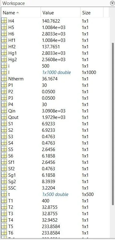
• Plots