Challenge

Project 2 - Rankine cycle Simulator

BBibek Joshi18 Apr 2022

MATLAB

AIM:

To create a Rankine Cycle Simulator.
To write a code to calculate the state points of the Rankine cycle based on user inputs.
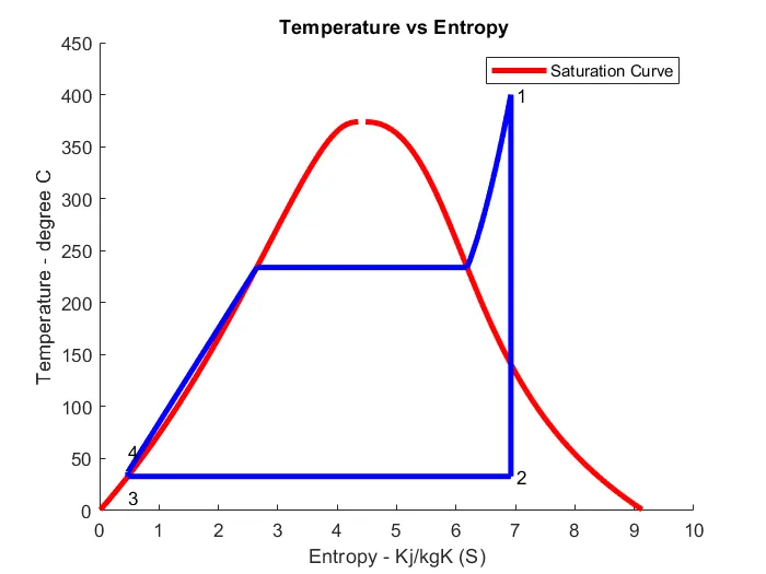
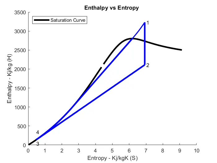
To plot the corresponding T-S and H-S plot for the given set of inputs.

INPUTS REQUIRED:

Turbine Inlet Temperature = 400 degrees C.
Turbine Inlet Pressure = 30 Bars.
Turbine Outlet Pressure = 0.05 Bars = Condenser Inlet pressure.

TO CALCULATE:

Net work done.
Back work ratio.

THEORY:

Rankine Cycle: The Rankine cycle or Rankine Vapor Cycle is the process widely used by power plants such as coal-fired power plants or nuclear reactors. In this mechanism, a fuel is used to produce heat within a boiler, converting water into steam which then expands through a turbine producing useful work. This process was developed in 1859 by Scottish engineer William J.M. Rankine. This is a thermodynamic cycle that converts heat into mechanical energy, which usually gets transformed into electricity by electrical generation.

Figure 1. A simple schematic with components for the Rankine Cycle.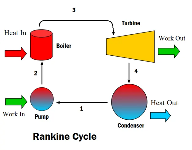

Figure 2. The pressure-volume (P-V) diagram of the Rankine cycle.

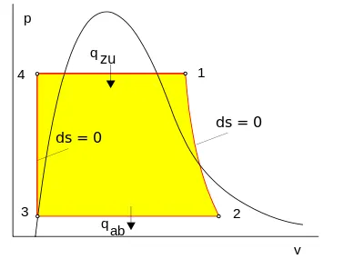
Pump: Compression of the fluid to high pressure using a pump (this takes work) (Figure 2: Steps 3 to 4)
Boiler: The compressed fluid is heated to the final temperature (which is at boiling point), therefore, a phase change occurs—from liquid to vapor. (Figure 2: Steps 4 to 1)
Turbine: Expansion of the vapor in the turbine. (Figure 2: Steps 1 to 2)
Condenser: Condensation of the vapor in the condenser (where the waste heat goes to the final heat sink (the atmosphere or a large body of water (ex. lake or river). (Figure 2: Steps 2 to 3)

The Rankine cycle closely describes the process by which steam engines commonly found in thermal power generation plants harness the thermal energy of a fuel or other heat source to generate electricity.
The efficiency of the Rankine cycle is limited by the high heat of vaporization by the fluid. The fluid must be cycled through and reused constantly, therefore, water is the most practical fluid for this cycle.

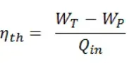
The thermal efficiency of the simple Rankine cycle and in terms of specific enthalpies can be calculated as:

A MATLAB PROGRAM FOR RANKINE CYCLE SIMULATOR.

% A MATLAB code to create a Rankine Cycle Simulator.
clear all
close all
clc

% Defining the 4 states of Rankine cycle.
disp ('RANKINE CYCLE');
disp ('1-2, is Constant pressure heat addition in the condenser');
disp ('2-3, is Isentropic Expansion in the turbine');
disp ('3-4, is Constant pressure heat rejection in the condenser');
disp ('4-1, is Isentropic compression in the pump');

% Providing the given data as input.
% Unit of Temperature is in Degree Celcius and Pressure is in Bar.

T1 = input ('Value of temperature at the turbine inlet, T1 = ');
p1 = input ('Value of pressure at the turbine inlet, P1 = ');
p2 = input ('Value of pressure at the condenser inlet, P2 = ');

% At state 1
% Extracting Enthalpy and Entropy at atate point 1.
h1 = XSteam('h_pT',p1,T1);
s1 = XSteam('s_pT',p1,T1);

% At state 2
% For isentropic expansion
s2 = s1;

% For Saturated liquid entropy
sf2 = XSteam('sL_p',p2);
% For Saturated liquid entropy
sg2 = XSteam('sV_p',p2);
x2 = (s2-sf2)/(sg2-sf2);
hf2 = XSteam('hL_p',p2);
hg2 = XSteam('hV_p',p2);
h2 = hf2+(x2*(hg2-hf2));

% At state 3
% Constant pressure heat rejection.
p3 = p2;
h3 = XSteam('hL_p',p3);
s3 = XSteam('sL_p',p3);

% At state 4

p4 = p1;
s4 = s3;

% To Calculate work done by the turbine (WT).
WT = h1 - h2;

% To calculate the workdone to run pump (WP).

v3 = XSteam('vL_p',p3);
WP = v3*(p4-p3)*100;
h4 = h3 + WP;

% Net work done (WN).

WN = WT-WP;

% Heat into the system.
Q_in = h1-h4;

% Heat out of the system.
Q_out= h2-h3;

% Thermal efficiency of the cycle.
T_eff =  (WN/Q_in)*100;

% Specific steam consumption ( SSC = mass flow rate / power).

SSC = (3600/WN);

% Back Work Ratio (BWR).
BWR = (WP/WT);

% Calculation of Temperature at the state points.

T3 = XSteam ('Tsat_p', p3);
T2 = T3;

Cp4 = XSteam('Cp_ps',p4, s4);
Cv4 = XSteam('Cv_ps',p4, s4);
k = Cp4/Cv4;
T4 = T3/((p3/p4)^((k-1)/k));

% Calculating Temperature, Entropy, Emthalpy at the vapour and liquid line for plotting.

T6 =  XSteam ('Tsat_p', p1);
s5 = XSteam('sL_p',p1);
s6 = XSteam('sV_p',p1);
h5 = XSteam('hL_p',p1);
h6 = XSteam('hV_p',p1);
T5 = T6;

% Plotting the saturation curve.

T = linspace (1,375,1000);
for i = 1:length(T)
    
    sf(i) = XSteam('sL_T',T(i));
    sg(i) = XSteam('sV_T',T(i));
    hf(i) = XSteam('hL_T',T(i));
    hg(i) = XSteam('hV_T',T(i));
end

% Plotting T-s diagram.

figure(1)
hold on
plot (sf,T,'r','linewidth',3)
plot (sg,T,'r','linewidth',3)
plot([s1 s2],[T1 T2],'b','linewidth',3)
plot([s2 s3],[T2 T3],'b','linewidth',3)
plot([s3 s4],[T3 T4],'b','linewidth',3)
plot([s4 s5],[T4 T5],'b','linewidth',3)
plot([s5 s6],[T5 T6],'b','linewidth',3)
sc1 = linspace(s6, s1, 1000);
for l = 1:length(sc1)
    Tc1(l) = XSteam('T_ps', p1, sc1(l));
end
plot(sc1, Tc1,'b','linewidth',3)
text (s1+0.1, T1,'1')
text (s2+0.1, T2,'2')
text (s3, T3-20,'3')
text (s4, T4+20,'4')
title ('Temperature vs Entropy ')
xlabel ('Entropy - Kj/kgK (S)')
ylabel ('Temperature - degree C')
legend ('Saturation Curve')


% Plotting h-s diagram.

figure(2)
hold on
plot (sf,hf,'k','linewidth',3)
plot (sg,hg,'k','linewidth',3)
plot([s1 s2],[h1 h2],'b','linewidth',3)
plot([s2 s3],[h2 h3],'b','linewidth',3)
plot([s3 s4],[h3 h4],'b','linewidth',3)

hc = linspace(h4, h5, 100);
for r = 1:length(hc)
    sch(r) = XSteam('s_ph', p1, hc(r));
end
plot(sch, hc,'b','linewidth',3)
plot([s5 s6],[h5 h6],'b','linewidth',3)

for m = 1:length(sc1)
    hc1(m) = XSteam ('h_ps',p1,sc1(m));
end
plot (sc1, hc1, 'b','linewidth',2)
text (s1+0.1, h1,'1')
text (s2+0.1, h2,'2')
text (s3, h3-100,'3')
text (s4, h4+200,'4')
title ('Enthalpy vs Entropy ')
xlabel ('Entropy - Kj/kgK (S)')
ylabel ('Enthalpy - Kj/kg (H)')
legend ('Saturation Curve','location','northwest')


% To display the result in the command Window. 

disp ('RESULTS');
p1 = p1;
T1 = T1;
p2 = p2;

disp('At State point 1');
n1 = sprintf('P1 is %.3f bar', p1);
disp(n1);

n2 = sprintf('T1 is %.3f C', T1);
disp(n2);

n3 = sprintf('h1 is %.3f Kj/kg', h1);
disp(n3);

n4 = sprintf('s1 is %.3f Kj/kgK', s1);
disp(n4);


disp('At State point 2');

n11 = sprintf('P2 is %.3f bar', p2);
disp(n11);

n21 = sprintf('T2 is %.3f C', T2);
disp(n21);

n31 = sprintf('h2 is %.3f Kj/kg', h2);
disp(n31);

n41 = sprintf('s2 is %.3f Kj/kgK', s2);
disp(n41);

disp('At State point 3');

n12 = sprintf('P3 is %.3f bar', p3);
disp(n3);

n22 = sprintf('T3 is %.3f C', T3);
disp(n3);

n32 = sprintf('h3 is %.3f Kj/kg', h3);
disp(n32);

n42 = sprintf('s3 is %.3f Kj/kgK', s3);
disp(n42);

disp('At State point 4');

n13 = sprintf('P4 is %.3f bar', p4);
disp(n13);

n23 = sprintf('T4 is %.3f C', T4);
disp(n23);

n33 = sprintf('h4 is %.3f Kj/kg', h4);
disp(n33);

n43 = sprintf('s4 is %.3f Kj/kgK', s4);
disp(n43);
n14 = sprintf('WT is %.3f Kj/kg', WT);
disp(n14);
n15 = sprintf('WP is %.3f Kj/kg', WP);
disp(n15);
n16 = sprintf('WN is %.3f Kj/kg', WN);
disp(n16);
n17 = sprintf('Thermal efficiency is %.2f Kj/kg', T_eff);
disp(n17);
n18 = sprintf('SSC is %.2f Kj/KWh', SSC);
disp(n18);
n19 = sprintf('Back Work Ratio is %.3f Kj/kg', BWR);
disp(n19);

EXPLANATION:

At first, 4 phases of the Rankine cycle were defined.
Given input data was loaded to the program.
XSteam data was used to extract water and vapor properties of Enthalpy, Entropy at specific Temperatures and Pressure.
Then the state point of the Rankine cycle was calculated using input data and XSteam data.
Thermodynamic relation was used to calculate the enthalpy of water " h1 = XSteam('h_pT',p1,T1); "
Entropy was also calculated " s1 = XSteam('s_pT',p1,T1); "
Thermodynamic relation was used to extract further state points and their data from XSteam.
Extracted data were used to calculate The Net work, Work done by the turbine, Work done to run the pump, Heat in, and Heat out.
Efficiency and Specific Steam Consumption (SSC) of the Rankine cycle were also calculated.
T, s, and h were extracted for vapor and water states for plotting.
For saturated liquid and gas, the saturation curve is plotted.
T vs s and h vs s plot is created using all the data calculated using the code.
All the calculated and extracted data were displayed on the command window using sprintf command.
As the code asks for user inputs, the output of the program depends upon user inputs.

RESULTS:

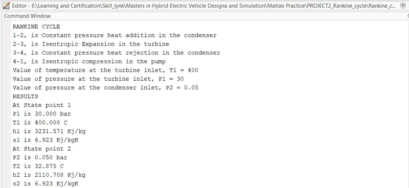
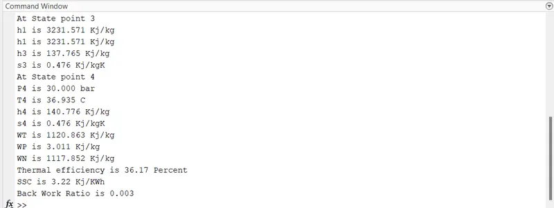
The Matlab code for the Rankine cycle simulation was run and Rankine cycle performance was observed.

Net work done (WN) = 1117.852 Kj/kg
Work done by Turbine (WT) = 1120.863 Kj/kg
Work done by Pump (WP) = 3.011 Kj/kg
Thermal efficiency is 36.17 Percent
SSC = 3.22 Kj/KWh
Back Work Ratio = 0.003

RESULTS ARE DISPLAYED IN THE COMMAND WINDOW.

PLOTS:

The plot between Temperature & Entropy and Enthalpy & Entropy is shown below.

ERROR FACED AND THEIR SOLUTIONS:

An invalid Expression error was shown in the command window. Typing error was found as a mistake in the syntax. Instead of Cv, it was CV.

The corrected syntax was used as shown below to rectify this error.
An invalid Expression error was shown in the command window. A bracket " ( " was missing in the syntax.

Later ( was added and syntax was error free. Corrected code is shown below.

CONCLUSION:

Hence, A MATLAB program was created and run to simulate the Rankine Cycle and to calculate the required thermodynamic data.

REFERENCES:

Project 2 - Rankine cycle Simulator

Ship work like this
in your own course.

Talk to a career counsellor

Ship work like thisin your own course.

Talk to a career counsellor

Ship work like this
in your own course.