Project 2 - Rankine cycle Simulator

AIM :- To create Rankine Cycle simulator using MatLab by using standard thermodyanamic library of steam table (XSteam).

OBJECTIVES :-

• To create a Rankine cycle simulator in MATLAB.
• To callculate all the state points using XSteam.
• To plot the T-S & H-S curve for given input of Rankine cycle.
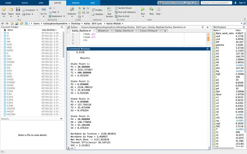
• To get output in the command window for each state points in cycle.

INTRODUCTION :-

The Rankine cycle is an idealized thermodynamic cycle describing the process by which certain heat engines, such as steam turbines or reciprocating steam engines, allow mechanical work to be extracted from a fluid as it moves between a heat source and heat sink. The Rankine cycle is named after William John Macquorn Rankine, a Scottish polymath professor at Glasgow University.

• Heat energy is supplied to the system via a boiler where the working fluid (typically water) is converted to a high pressure gaseous state (steam) in order to turn a turbine.
• After passing over the turbine the fluid is allowed to condense back into a liquid state as waste heat energy is rejected before being returned to boiler, completing the cycle.
• Friction losses throughout the system are often neglected for the purpose of simplifying calculations as such losses are usually much less significant than thermodynamic losses, especially in larger systems.

Components :-

(1) PUMP :-

• A pump is a mechanical device, that is used to pick up water from low-pressure level to high-pressure level. Basically, the pump changes the energy flow from mechanical to the fluid.
• The liquid condensate leaving the condenser at the state 1 is pumped to the operating pressure of the boiler. The pump operation is considered isentropic.

(2) BOILER :-

• A boiler is a closed vessel in which fluid (generally water) is heated. The fluid does not necessarily boil. The heated or vaporized fluid exits the boiler for use in various processes or heating applications, including water heating, central heating, boiler-based power generation, cooking and sanitation.
• The heat is supplied in the working fluid (feed water) in the boiler and thus vapour is generated. The vapour leaving the boiler either at saturated at the stage 3 or superheated at the stahe 3, depending upon the amount of heat supplied by thr boiler.

(3) TURBINE :-

• A turbine is a machine or engine which uses a staem of air, gas, water, or steam to turn a wheel and produce power.
• The vapour leaving the boiler enters the turbine, where it expands isentropically to the condenser pressure at state 4. The work produced y the turbine is rotary (shaft) work and is used to drive an electric generator or machine.

(4) CONDENSOR :-

• A condenser in its simplest terms is a heat transfer device which reduces a thermodynamic fluid from its vapor phase to its liquid phase.
• The condenser is attached at the exit of the turbine. The vapour leaving the turbine is wet vapour and is condensed completely in the condenser to the state 1, by giving its latent heat to some water other coolling fluid like water.

DESCRIPTION :-

In an ideal Rankine cycle the pump and turbine would be isentropic i.e. the pump and turbine would generate no entropy and hence maximize the net work output. Processes 1–2 and 3–4 would be represented by vertical lines on the T-s diagram and more closely resemble that of the carnot cycle. The Rankine cycle shown here prevents the state of the working fluid from ending up in the superheated vapor region after the expansion in the turbine, which reduces the energy removed by the condensers.

The actual vapor power cycle differs from the ideal Rankine cycle because of irreversibilities in the inherent components caused by fluid friction and heat loss to the surroundings; fluid friction causes pressure drops in the boiler, the condenser, and the piping between the components, and as a result the steam leaves the boiler at a lower pressure; heat loss reduces the net work output, thus heat addition to the steam in the boiler is required to maintain the same level of net work output.

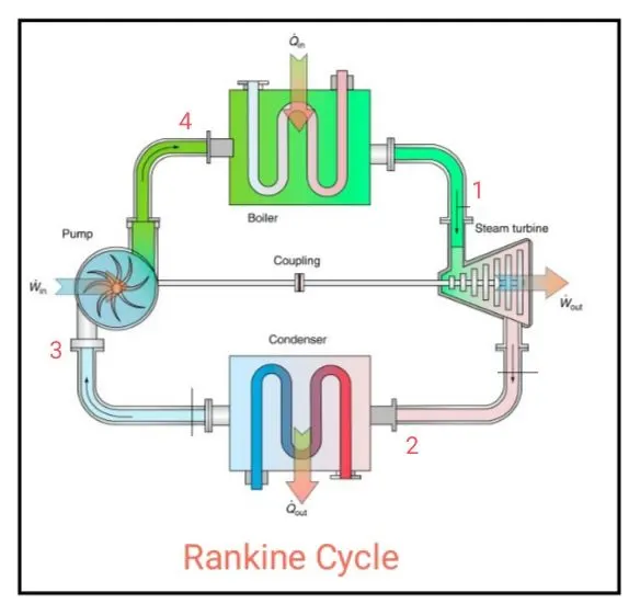
There are four processes in the Rankine cycle. The states are identified by numbers in the T-S diagram.

(1) Process 1–2: The working fluid is pumped from low to high pressure. As the fluid is a liquid at this stage, the pump requires little input energy.

• Process 1-2 is isentropic compression.

(2) Process 2–3: The high-pressure liquid enters a boiler, where it is heated at constant pressure by an external heat source to become a dry saturated vapour. The input energy required can be easily calculated graphically, using an enthaply-entropy chart (h-s chart/Mollier Diagram), or numerically, using steam tables or software.

• Process 2-3 is constant pressure heat addition in boiler.

(3) Process 3–4: The dry saturated vapour expands through a turbine, generating power. This decreases the temperature and pressure of the vapour, and some condensation may occur. The output in this process can be easily calculated using the chart or tables noted above.

• Process 3-4 is isentropic expansion.

(4) Process 4–1: The wet vapour then enters a condeser, where it is condensed at a constant pressure to become a saturated. liquid.

• Process 4-1 is constant pressure heat rejection in condenser.

MAIN PROGRAM :-

PROCEDURE OF PROGRAM :-

• The code starts with clear all, close all, clc where,
• 'clear all' command is used to clear the data stored in the workspace.
• 'close all' command is used to close all plots and figures.
• 'clc' command is used to clear the commaand the window.
• The creastion of Rankine cycle simulator starts with some inpput value which are required to calculate th other state point in cycle eventually.
• The Rankine cycle process is displayed in the command window and then inputs are entered which are inlet pressure fr turbine, temperature at turbine inlet and pressure at condenser.
• Then we are using XSteam function file for reading state point.First we get the value of enthalpy and entropy at state point 1 from the XSteam function file.
• As process from 1-2 is isentropic compression the entropy at point 1 equal to point 2.The term (s_pT,p1,T1) refers to entropy at pressure and temperature point 1.
• The term 'sg' and 'sf' are referred to saturated liquid and vapour entropy respectively. This value is used to claculate other function according to mathematically relations.
• Similarly, other points are taken from XSream function file which are necessary to calculate other parameters. After that work done in turbine & pump are calculated for further getting the net work done Rankine Cycle.
• After calculating the net work done the efficiency of the Rankine cycle is calculated by a locomotive cylinders per unit of output of work done.
• Then temperature at each point of cycle is calculated using input taken from start of the program and data taken fro XSteam file.
• for given temeprature range from lower to higher entropy points are calculated to create the T-S plot. Similarly, another for loop is used to create the saturation curve in each plot.
• Then plotting is done for T-S and H-S graph of Rankine cycle and each state point value has been put in ommand window.

RESULTS/OUTPUT :-

Fig 1- T-S Digram of Rankine Cycle Fig 2- H-S Digram of Rankine Cycle

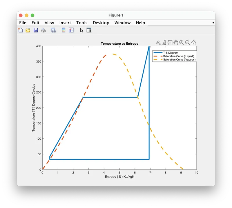
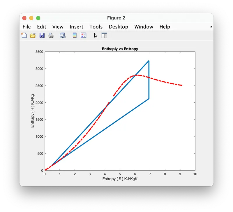
Fig 3- Output results of Program

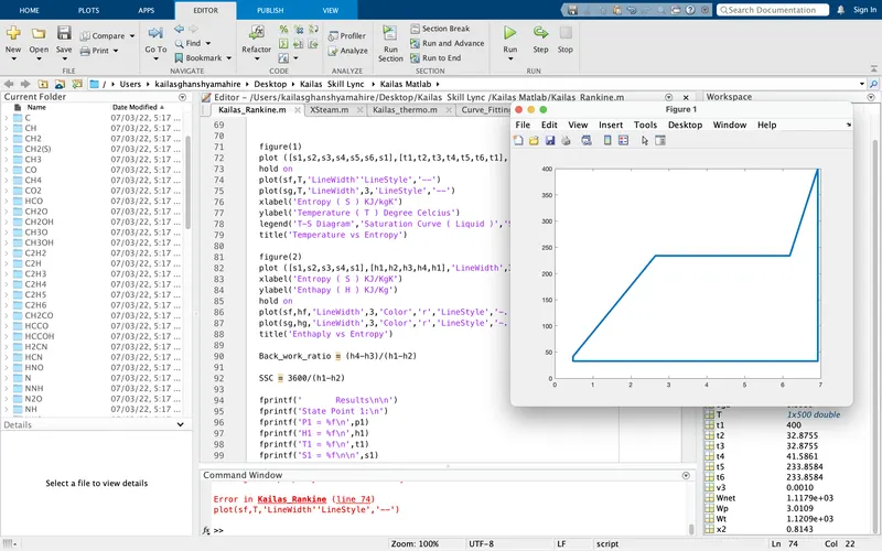
ERROR :-

Saturation Curve not ontained due to linewidth not mention in line No. 74.

CONCLUSION :-

• After this program we can conclude that MATLAB program for rankine cycle was computed and this code helps to design the power plant operating condition by which the plant efficiency can be increased and specific steam consumption can be decreased.