Challenge

Week 3 - Solving second order ODEs

KKailas Ahire12 Feb 2022

AIM :- To solve the second order ODE function using MatLab which depites the motion of the pendulum and to create an animation of the same.

INTRODUCTION :-

A Pendulum is a weight suspended from a pivot so that it can swing freely. When a pendulum is displaced sideways from its resting, equilibrium position, it is subject to a restoring force due to gravity that will accelerate it back toward the equilibrium position. When released, the restoring force acting on the pendulum's mass causes it to oscillate about the equilibrium position, swinging back and forth. The time for one complete cycle, a left swing and a right swing, is called the period. The period depends on the length of the pendulum and also to a slight degree on the amplitude, the width of the pendulum's swing

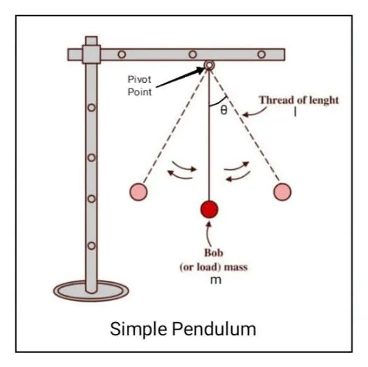
OBJECTIVE :- To write a program that solves the following ODE. This ODE represents the equation of motion of a simple pendulum with damping.

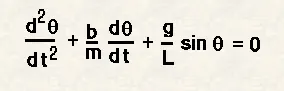
In the above equation,

g = Gravity (m/s^2)
L = Length of pendulum (m)
m = Mass of the ball (Kg)
b = damping Co-efficient

Given Data :-

Length (l) = 1 meter,
Mass (m)= 1 Kg,
Damping Co-efficient (b) = 0.05 (Unit less Entity),
Gravitational Acceleration (g) = 9.81 m/s^2,
Tiime Span (t) = 0-20 Sec,
Angular displacement = 0 rad,
Angular Velocity = 3 rad/Sec at time t = 0.

FUNCTION CODE PROGRAM :-

% ODE Function

function [dtheta_dt] = Kailas_func(t,theta,b,g,l,m)

theta1 = theta(1)

theta2 = theta(2)

dtheta1_dt = theta2;

dtheta2_dt = -(b/m)*theta2 - (g/l)*sind(theta1);

dtheta_dt = [dtheta1_dt; dtheta2_dt];

end

EXPLAINATION OF FUNCTION CODE :-

In this function program, the second order equation (ODE) is simplified to the first order ODE by introducing the term theta1 & theta2
Then theta1 & theta2 is differentiated and the dtheta_dt gives a column matrix.

MAIN PROGRAM :-

% Prgoram for Simple Pendulum

clear all

close all

clc

b = 0.05; % Damping Co-efficient

g = 9.81; % Gravitational Acceleration (m/s^2)

l = 1.0; % Length of Pendulum (m)

m = 1.0; % Mass (Kg)

% Initial condition

theta_0 = [0;0.3];

% Time points

t_span = linspace(0,20,100);

% Solve ODE

[t,results] = ode45(@(t,theta) Kailas_func(t,theta,b,g,l,m),t_span,theta_0);

% Plotting

% Figure(1)

plot(t,results(:,1),'LineWidth',3)

hold on

plot(t,results(:,2),'LineWidth',3)

title('Pendulum Oscillation Graph')

xlabel('Time (Sec)')

ylabel('Velocity (Red) & Displacement (Blue)')

% Animation

ct = 1;

for i = 1:length(results(:,1))

x0 = 0;

y0 = 0;

x1 = l*sin(results(i,1)+pi);

y1 = l*cos(results(i,1)+pi);

% figure (2)

plot([x0 x1],[y0 y1],'-o','MarkerSize',15,'MarkerFaceColor','r','MarkerEdgeColor','r','LineWidth',4)

axis([-2 2 -2 2])

hold on

plot([-1 1],[0 0],'LineWidth',4,'Color','[0 0.3 0]')

M(ct) = getframe(gcf)

hold off

ct = ct + 1;

end

% Movie & Videofile

movie(M)

v_f = VideoWriter ('Challenge_Pendulum.avi','Uncompressed AVI')

open (v_f)

writeVideo (v_f,M)

close (v_f)

EXPLAINATION OF MAIN PROGRAM :-

The code starts with clear all, close all, clc where,
'clear all' command is used to clear the data stored in the workspace.
'close all' command is used to close all plots and figures.
'clc' command is used to clear the commaand the window.
In the above program, the fixed parameters are length, mass, damping Co-efficient and Gravitational accelaration. Time and angle given as the initial condition.
In the t_span command, 100 values are taken in between 0 - 20 Sec time period.
Using the ode45 command ODE function introduced.
Using the plot command Velocity and displacement is plotted in the Y-axis against time in the X-axis.
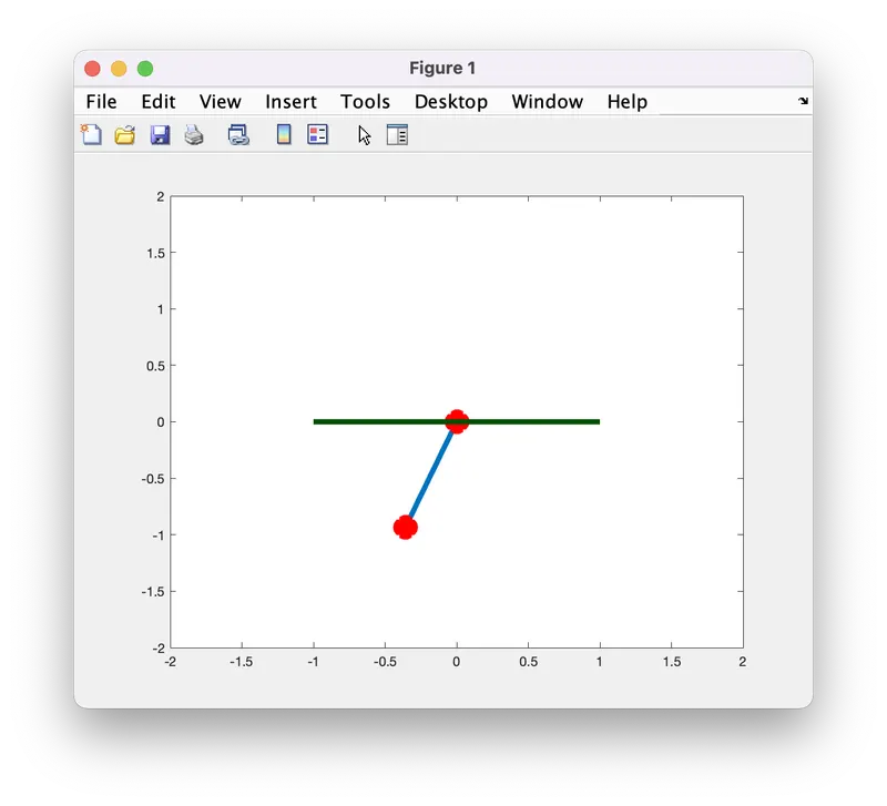
Using the For_End loop command the mass at various points and various times are marked in the graph.
All figure assigned to a variable M, one at a time using ct followed by termination of for loop.
Lastly, movie cammand is used to combine all the figures saved in the M file to make an animation or movie and thereafter saving it in .avi format.

RESULTS :-

OUTPUT OF PROGRAM

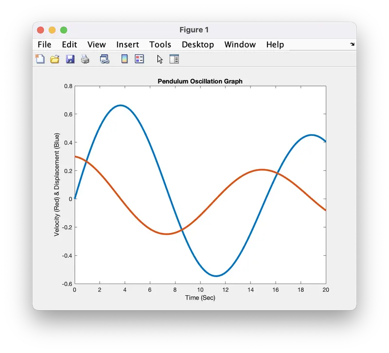
Graph for the velocity v/s time which shows Displacement and Angular velocity.
The Dsipalcement (Blue color) and Angular velocity (Red color) is decreasing by the increased time, this is duw to the introduction of Damper i.e Damping Co-efficient which absorbs the vibrations to make the body in equilibrium position

GOOGLE DRIVE ANIMATION LINK :- https://drive.google.com/file/d/1sU_kdCR6Sk6cp0299QeXUVy7FuJ-FL51/view?usp=sharing

CONCLUSION :-

After this program, we about ODE45 solver aniamted video the simple pendulum using ODE45 solver where the second order eqauation is reduced to a first order differential equation where it is easy to solve the given equation.
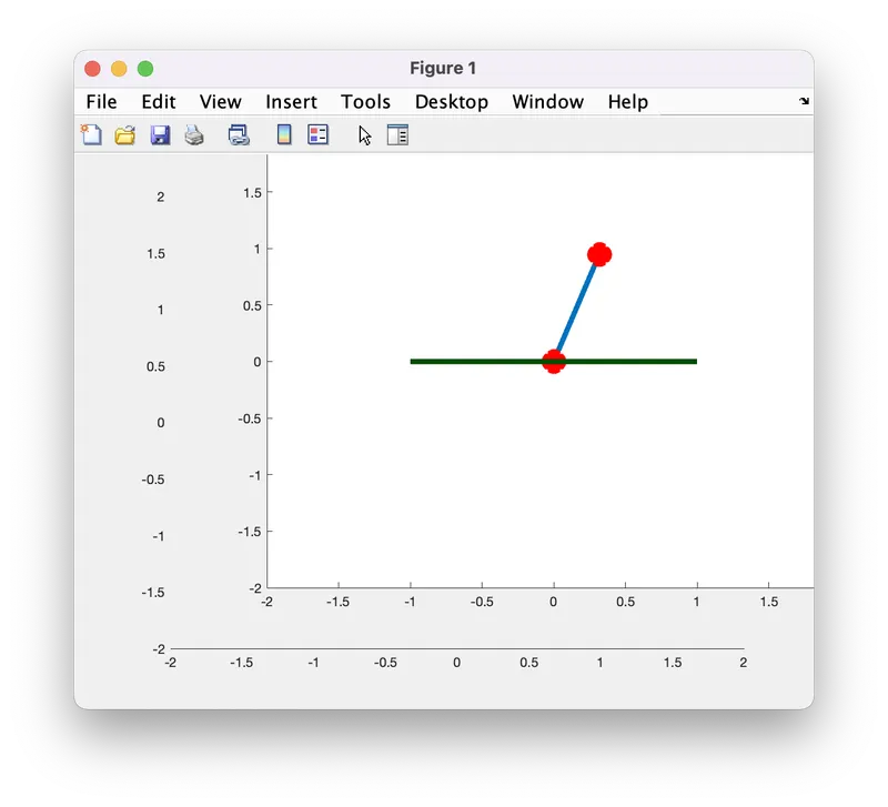
The animation of simple pendulum created.

ERRORS :-

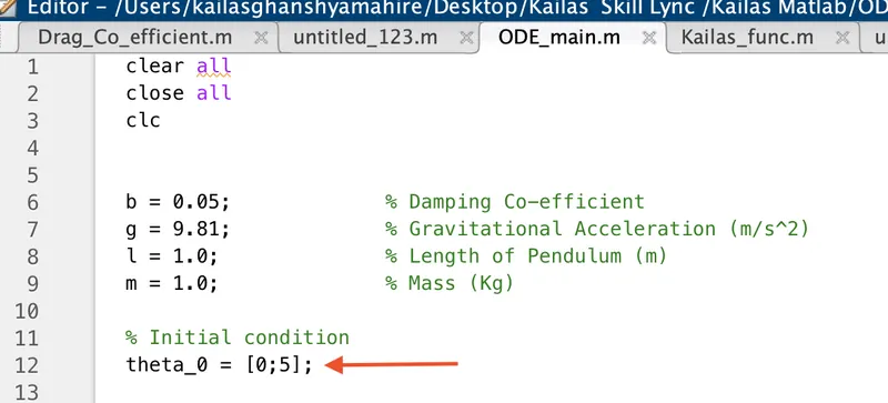
In initial condition theta was entered by 0;5 which was wrong due to that pendulum was not properly oscillating.

Thank You ...

Week 3 - Solving second order ODEs

Ship work like this
in your own course.

Talk to a career counsellor

Ship work like thisin your own course.

Talk to a career counsellor

Ship work like this
in your own course.