Project 2 - Rankine cycle Simulator
AIM:
- Create a Rankine Cycle Simulator using OCTAVE/MATLAB.
PROCEDURE
RANKINE CYCLE:
The Rankine cycle or Rankine Vapor Cycle is the process widely used by power plants such as coal-fired power plants or nuclear reactors. In this mechanism, a fuel is used to produce heat within a boiler, converting water into steam which then expands through a turbine producing useful work.
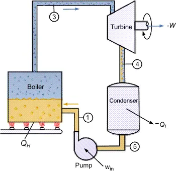
In a Rankine cycle, high-pressure liquid water (1) enters a boiler where it is heated to saturation temperature (2), vaporized, and superheated (3). The superheated steam is fed to a turbine, where it expands and generates mechanical work. The steam exits the turbine at a lower pressure and temperature as either superheated steam or steam with a vapor quality (4). After the steam is condensed (5), a pump compresses the liquid water to high pressure (1). Select “P-H diagram” to see the cycle on a pressure-enthalpy diagram. Use sliders to select the inlet pressure to the turbine P3 and one of four outlet pressures P4. Use a slider to vary the turbine efficiency ηT, which is the ratio of work produced by the turbine to the work produced by a reversible turbine between the same inlet and outlet pressures. The irreversible turbine pathway (ηT < 1) is the dashed black line on the P-H diagram; the reversible turbine pathway is the orange dashed line. Select “Rankine cycle” to view a schematic of the cycle, and select “turbine” to show the inlet and outlet conditions for the turbine and the work generated.
PROCESSES:
- Process 1–2: The working fluid is pumped from low to high pressure. As the fluid is a liquid at this stage, the pump requires little input energy. Process 1-2 is isentropic compression.
- Process 2–3: The high-pressure liquid enters a boiler, where it is heated at constant pressure by an external heat source to become a dry saturated vapor. The input energy required can be easily calculated graphically, using an enthalpy-entropy chart (H-S CHART) OR (MOLLIER DIAGRAM), or numerically, using Steam tables or software. Process 2-3 is constant pressure heat addition in the boiler.
- Process 3–4: The dry saturated vapor expands through a Turbine, generating power. This decreases the temperature and pressure of the vapor, and some condensation may occur. The output in this process can be easily calculated using the chart or tables noted above. Process 3-4 is isentropic expansion.
- Process 4–1: The wet vapor then enters a Condensor, where it is condensed at a constant pressure to become a Saturated liquid. Process 4-1 is constant pressure heat rejection in the condenser.
HOW IT IS CALCULATED?
absolute temperature scale
Fahrenheit scale is called the Rankine (°R) scale. These scales are related by the equations K = °C + 273.15, °R = °F + 459.67, and °R = 1.8 K. Zero in both the Kelvin and Rankine scales is at absolute zero.
EQUATIONS:
n general, the efficiency of a simple Rankine cycle can be written as

Each of the next four equations is derived from the Energy and mass balance for a control volume.  defines thermodynamic efficiency of the cycle as the ratio of net power output to heat input. As the work required by the pump is often around 1% of the turbine work output, it can be simplified.




When dealing with the efficiencies of the turbines and pumps, an adjustment to the work terms must be made:


COMPONENTS.
A Rankine cycle power system is a heat engine converting thermal energy into work. Similar to the vapor compression heat pump, it comprises four main components: a boiler (sometimes called the evaporator), a turbine, a condenser, and a pump
CODE FOR RANKINE CYCLE SIMULATOR:
clear all
close all
clc
fprintf(' SIMULATOR OF RANKINE CYCLE nn')
fprintf('1-2 Isentropic Expansion in the Turbinen')
fprintf('2-3 Constant Pressure Heat Rejection by the Condensern')
fprintf('3-2 Isentropic Compression in the Pumpn')
fprintf('4-1 Constant Pressure Heat Addition by the Boilernn')
%inputs
P1 = input('Enter the Pressure at the Turbine Inlet (in bar): ');
T1 = input('Enter the Temperature at the Turbine inlet (in Degree celsius): ');
P2 = input('Enter the Pressure at the Condenser (in bar): ');
disp(' RESULTS')
%getting Cp and cv values from Xsteam
%Cp and Cv assumed to not change with temperature to make problem simple
% for vapur
high_cpV= XSteam('CpV_p', P1);
low_cpV=XSteam('CpV_p', P2);
high_cvV=XSteam('CvV_p', P1);
low_cvV=XSteam('CvV_p', P2);
% for liquid
high_cpL= XSteam('CpL_p', P1);
low_cpL=XSteam('CpL_p', P2);
high_cvL=XSteam('CvL_p', P1);
low_cvL=XSteam('CvL_p', P2);
%Getting important parameters from Xsteam
%for high pressure
T1s = XSteam('Tsat_p', P1);
S1g = XSteam('sV_p', P1);
S1f = XSteam('SL_p', P1);
S1fg = S1g - S1f;
H1f = XSteam('hL_p', P1);
H1g = XSteam('hV_p', P1);
H1fg = H1g - H1f;
%for low pressure
S2g = XSteam('sV_p', P2);
S2f = XSteam('SL_p', P2);
S2fg = S2g - S2f;
T2s = XSteam('Tsat_p', P2);
H2f = XSteam('hL_p', P2);
H2g = XSteam('hV_p', P2);
H2fg = H2g - H2f;
%% State point 1
disp('At state point 1:')
fprintf('P1 is : %f Barn', P1)
fprintf('T1 is : %f Deg celsiusn', T1)
H1 = XSteam('h_pt', P1, T1);
fprintf('H1 is : %f kJ/kgn', H1)
S1 = XSteam('s_pt', P1, T1);
fprintf('S1 is : %f kJ/kgKnn', S1)
%% State point 2
disp('At state point 2:')
fprintf('P2 is : %f Barn', P2) %P2 input already taken
S2 = S1;
fprintf('S2 is : %f kJ/kgKn', S2)
%predicting location of point 2 in T-s
if(S2<=S2g)
 X2 = (S2 - S2f) / (S2fg); % Dryness Fraction at state point 2
else
 X2=1;
end
fprintf('X2 is :%f n', X2)
%calculating T2 for superheat or wet or dry wherever it lies
if(X2<1)
 T2=T2s;
else
 %t2 cal by s2=s2g+low_cpV*(log(T2/T2s))
 T2=(T2s+273.15)*exp((S2-S2g)/low_cpV) ; %2 in superheated region
 T2=T2-273.15;
end
fprintf('T2 is : %f Deg celsius n', T2)
if(X2<1)
 H2 = H2f + X2 * H2fg;
else
 H2=H2g+ low_cpV*(T2-T2s);
end
fprintf('H2 is : %f kJ/kgn', H2)
%% State point 3
%Assuming no subcooling in condensor
disp('At state point 3:')
P3 = P2;
fprintf('P3 is : %f Barn', P3)
V3 = XSteam('vL_p', P3);
T3 = T2s; %no subcooling assumed
fprintf('T3 is : %f Deg celsiusn', T3)
H3 =H2f;
fprintf('H3 is : %f kJ/kgn', H3)
S3 =S2f;
fprintf('S3 is : %f kJ/kgKnn', S3)
%% State point 4
disp('At state point 4:')
P4 = P1;
fprintf('P4 is : %f Barn', P4)
S4 = S3;
fprintf('S4 is : %f kJ/kgKn', S4)
Wp = V3 * (P4 - P3) * 100;
H4 = Wp + H3;
fprintf('H4 is : %f kJ/kgn', H4)
% to cal T4 s4=s3=sf1-high_cpL*ln(t1s/t4)
term=exp((S1f-S4)/high_cpL); %Use exp instead of Exp to take input as double
T4= T1s/term;
fprintf('T4 is : %f Deg celsius nn', T4)
%% Work done, heat, SSC and efficiency calculations
Wt = H1 - H2;
fprintf('Work by turbine is : %f kJ/kgn', Wt)
fprintf('Work by compressor is : %f kJ/kgn', Wp)
Wnet = Wt - Wp;
fprintf('Net Wok done is : %f kJ/kgn', Wnet)
Qin = H1 - H4;
eff_thermal = Wnet / Qin ; % Effieciency
fprintf('Thermal efficiency is : %f', eff_thermal); disp('%')
SSC = 3600 / Wt; % Specific steam consuption
fprintf('S.S.C is : %f kg/kWh ', SSC)
%% Calculation for plotting Liquid and Vapour lines
%
% <<FILENAME.PNG>>
%
temp = linspace(1, 373, 500);
for i = 1 : length(temp)
 H_L(i) = XSteam('hL_T', temp(i));
 H_V(i) = XSteam('hV_T', temp(i));
 S_L(i) = XSteam('sL_T', temp(i));
 S_V(i) = XSteam('sV_T', temp(i));
end
%% Ploting T - S and H - S Diagrams
figure(1) % T-S
hold on
plot([S1 S2], [T1 T2], 'r', 'linewidth', 1)
text(S1,T1,' 1')
text(S2,T2,' 2')
plot([S2 S2g], [T2 T2s], 'r', 'linewidth', 1)
text(S2g,T2s,' 2s')
plot([S2g S3], [T2s T3], 'r', 'linewidth', 1)
text(S3,T3,' 3')
plot([S3 S4], [T3 T4], 'r', 'linewidth', 1)
text(S4,T4,' 4')
plot([S4 S1f], [T4 T1s], 'r', 'linewidth', 1)
text(S1f,T1s,' 4s')
plot([S1f S1g], [T1s T1s], 'r', 'linewidth', 1)
text(S1g,T1s,' 1s')
plot([S1g S1], [T1s T1], 'r', 'linewidth', 1)
plot(S_L, temp, 'b', 'linestyle','--','linewidth', 1)
plot(S_V, temp, 'b', 'linestyle','--','linewidth', 1)
%marking direction
text(S1,(T1+T2)/2,'vee','HorizontalAlignment','center','color','r')
text((S2g+S2f)/2,T3,'langle','color','r')
text(S3,(T3+T4)/2,'wedge','HorizontalAlignment','center','color','r')
text((S1f+S1g)/2,T1s,'rangle','color','r')
title('T-S Diagram of Ideal Rankine Cylce')
ylabel('Temprature (degC)')
xlabel('Specific Entropy (kJ/kgK)')
figure(2) % H-S
5/7
hold on
plot([S1 S2], [H1 H2], 'r', 'linewidth', 1);
text(S1,H1,' 1')
plot([S2 S3], [H2 H3], 'r', 'linewidth', 1);
text(S2,H2,' 2')
plot([S3 S4], [H3 H4], 'r', 'linewidth', 1);
text(S3,H3,' 3')
plot([S4 S1], [H4 H1], 'r', 'linewidth', 1);
text(S4,H4,' 4')
plot(S_L, H_L, 'b','linestyle','--', 'linewidth', 1.5)
plot(S_V, H_V, 'b','linestyle','--', 'linewidth', 1.5)
title('H-S Diagram', 'FontSize', 15)
ylabel('Specific Enthalpy (kJ/kg)')
xlabel('Specific Entropy (kJ/kgK)')
OUTPUT:
 SIMULATOR OF RANKINE CYCLE nn1-2 Isentropic Expansion in the Turbinen2-3 Constant Pressure Heat Rejection by the Condensern3-2 Isentropic Compression in the Pumpn4-1 Constant Pressure Heat Addition by the BoilernnEnter the Pressure at the Turbine Inlet (in bar): 44
Enter the Temperature at the Turbine inlet (in Degree celsius): 583
Enter the Pressure at the Condenser (in bar): 5.38
 RESULTS
At state point 1:
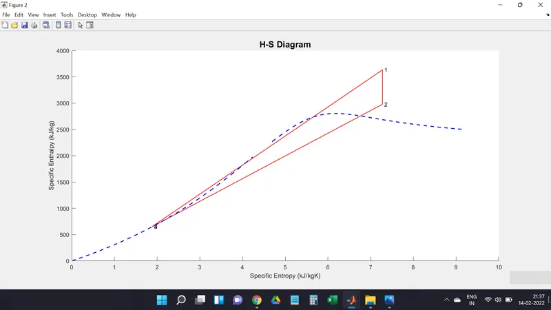
P1 is : 44.000000 BarnT1 is : 583.000000 Deg celsiusnH1 is : 3632.435734 kJ/kgnS1 is : 7.278301 kJ/kgKnnAt state point 2:
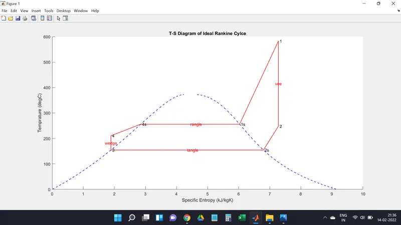
P2 is : 5.380000 BarnS2 is : 7.278301 kJ/kgKnX2 is :1.000000 nT2 is : 248.169455 Deg celsius nH2 is : 2979.515084 kJ/kgnAt state point 3:
P3 is : 5.380000 BarnT3 is : 154.616272 Deg celsiusnH3 is : 652.214783 kJ/kgnS3 is : 1.888715 kJ/kgKnnAt state point 4:
P4 is : 44.000000 BarnS4 is : 1.888715 kJ/kgKnH4 is : 656.446420 kJ/kgnT4 is : 210.781882 Deg celsius nnWork by turbine is : 652.920650 kJ/kgnWork by compressor is : 4.231637 kJ/kgnNet Wok done is : 648.689013 kJ/kgnThermal efficiency is : 0.217974%
S.S.C is : 5.513687 kg/kWh
ans =

    0.7143

>>
PLOTS:
T-S DIAGRAM.
H-S DIAGRAM.
REFERENCES:
2) https://en.wikipedia.org/wiki/Rankine_cycle#The_four_processes_in_the_Rankine_cycle
3) USING THE REFERENCES OF THE GIVEN X STREAM FILE.