Project 2 - Rankine cycle Simulator

Rankine cycle :-

Rankine cycle is an idenlizd thermodynamics cycle or headt engine in which a fuel is used to produce heat within a bolier , converting water into steam which then expands through a bolier turbin peoducing useful work. this processes was developed in 1859 by scottish engineer william j.m rankine. it is cycle which convert heat into mechanical energy which usually is converted into electrical energy.

1. in this project an idealize cycle is simulated. hence negelecting losses.

2.

3. Rankine cycle is derived out of carnot cycle its power depends on the temperature difference between the heat source and a cold source. the more the difference the more mechanical power can be efficiently extract out of heat energy.

4. since idea cycle are only in theory , efficieny of rankine cycle is limited high heat of vapourization of the work fluid , friction losses .

5. water usually the fluid of choice due to its favorable properties, such as its non-toxic and unreactive chemistry , abundance , and low cost aswell as it thermodynamics properties. by condensing the work steam vapour to a liquid the pressire at a turbine outlet is lowered and the energy required by the feed pump consumed to a higher efficiency for the cycle. the benefit of this is offset by the low temperature of steam admitted to the turbine.

. Processes and Working:

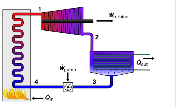
there are four process in the rankine cycle (order amybe varied)

1. process1-2 : isentropic expension in the turbine.

2. process2-3 : constant pressure heat rejection in condenser

3. process3-4 : isentropic compression in the pump

4. process4-1 : constant pressure heat addition in the boiler

working for the rankine cycle simulator

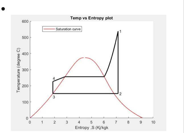
1. in process1-2 , the dry saturated vapour expands through a turbine, generating power. this decresses the temperature and pressure of the vapour, and some condensation may occur.

2. process2-3 , the vapour liquid mixture leaving the turbine (2) is condensed at low pressure , usually in a surface condensers using cooling water. in well designed and maintainedcondensers , the pressure of the vapour is well below atmospheric pressure, approaching the saturation pressure of the operating fluid at the coling water temperature.

3. process3-4 , the pressure of the condensate is raised in the feed pump. because of the specific volume of liquid the pump work is relativetly small and the neglected in thermodynamic calculation.

4. process4-1 , high pressure liquid enters the boiler from the feed pump (4) and is heats to the saturation temperature (on the saturation curve). further addition of energy causes evaporation of the liquid unit it is fully converted to saturated steam(1) or superheated(1).

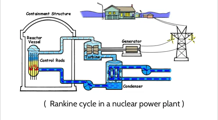
Elaborating (ranking cycle paragraph point v)

the water condenses in the condenser, waste heat is given off in the from of tower . this waste heat is nexessary in any thermodynamics cycle. due to this condensation step , the pressure at the turbine outlet is lowered this means the pump required less work to compree the water-resulting in higher overall efficiencies.

matlab project program:

%% Rankine cycle simulator

%%%%%%%%%%%%%%%%%%%%%%%%%%%%%%%%%

%%%%%%%%%%%%%%%%%

% objective of this program is to simulate the rankine cycle

% plotting t-s and h-s diagram using data from xsteam data

% water and steam properties according to IAPWS IF-97

clear all

close all

clc

%%

disp(' RANKINE CYCLE ');

% displaying

disp(' 1-2 is isentropic expansion in the turbine "0;

disp(' 2-3 is constant pressure heat removal in the condenser');

disp(' 3-4 is isentropic compression in the pump');

disp('4-1 is constant pressure heat addition in the boiler');

%%

%obtaining the input data

p1 = input('nvalue of pressure at turbine inlet, p1(in bar) = '):

T1 = input ('nvalue of temperature at turbine inlet,

T1 = (in degree.c) = ');

p2 = input ('nvalue of temperature at condenser inlet , p2( in bar) + ');

%%

% extracting data_defining variables

% state 1

h1 = xsteam('h_pT', p1, T1); % extracting ent

halpy at state pt 1

s1 = xsteam ('s_pT', p1, T1); % similarly

% state 2

s2 = s1;

ansion % isentropic exp

sf2 = xsteam ('sv_p',p2); % saturated liqu

id entropy

sg2 = xsteam ('sv_p' , p2); % saturated vapo

ur entropy

x2 = (s2-sf2)/sg2-sf2);

hf2 = xsteam ('hl_p', p2);

hg2 = xsteam ('hv_p',p2);

h2 = hf2 + (x2*(hg2-hf2));

% state 3

p3 = p2; % constant press

ure heat rejection in condenser

s3 = xsteam ('sl_p', p3);

h3 = xsteam ('hl_p', p3);

% state 4

s4 = s3;

p4 = p1;

%%

% work done by turbine

wt = h1 - h22;

% work done to run pump

v3 = xsteam ('vl_p', p3);

wp = v2*(p4 - p3)*100;

h4 = h3 + wp;

%net work

Wnet = wt - wp;

%heat into the system

Qin = h1 - h4;

%thermal efficiency

eff = (Wnet/Qin)*100;

%specific steam consumtion

%scc = mass flow rate/power

scc = (3600/Wnet);

%%

%calculating temperature at the state points

T3 = xsteam (' Tsat_p', p3);

T@ = T3;

cp4 = xsteam( 'cp_ps' , p4, s4);

cv4 = xsteam(' cv_ps' , p4, s4);

k = cp4/cv4;

T4 = T3/((p3/p4)^((k-1)/k));

%calculating temperature, entropy and enthalpy at the vapour and liquid

%line for plotting

T6 = xsteam('Tsat_p' , p1);

S5 = xsteam('sl_p' , p10;

S6 = xsteam('sv_p' , p1);

h5 = xsteam('hl_p' , p1);

h6 = xsteam('hv_p' , p1);

h5 = T6;

%%

%ploting the saturation curve

t = linespace (1,375,1000);

for i = 1:lenght(T)

sf(I) = xsteam('sl_T' , T(I));

sg(I) = xsteam('sv_T' , T(I));

hf(I) = xsteam('hl_T' , T(I));

hg(I) = xsteam('hv_Y' , T(I));

ens

% plotting t-s diagram

figure (1)

hold on

plot(sf, t, 'r'r,'linewidth' , 1)

plot(sg, t, 'r', 'linewidth' , 1)

plot([s1 s2] , [T1 T2], 'k', 'linewidth' , 2)

plot([s2 s3] , [T1 T3], 'k' , 'linewidth' ,2)

plot([s3 s4] , [T3 T4], 'k' , 'linewidth', 2)

plot([s4 s5] , [T4 T5], 'k' , 'linewidth' , 2)

plot([s5 s6] , [T5 T6], 'k' , 'linewidth' , 2)

sc1 = linspace (s6, s1, 1000);

for l = 1:lenght(sc1)

Tc1(l) = xsteam( 'T_ps' , p1, sc1(l));

end

plot(sc1, tc1, 'k', 'linewidth' ,2)

text(s1+0.1, t1, '1')

text(s2+0.1,t2, '2')

text(s3,t3-20, '2')

text(s4, t4+20, '4')

title('temp vs entropy plot')

xlabel('entropy ,s (kj/kgk')

ylabel('temperature (degree c) ')

legend('saturation curve')

%%

%plotting h-s diagram

figure(2)

hold on

plot(sf, hf, 'r', 'linewidth' , 1)

plot(sg, hg, 'r', 'linewidth' , 1)

1. xsteam data is used to extract steam and water properties of enthalpy, entropy at specific pressure and temperature for sat liquid sat vapour condition

2. the profram required the input of pressure at state point 1 the temperature at same point and temperature at condenser inlet point 2

3. the help of this inlet and from xsteam data, the program calculation all the state points of the rankine cycle.

4.the xsteam data rankine cycle.

5. h1 = xsteam ('h_pT' , p1,T1); (returen the enthalpy of water at given pressure and temperature in bar and degC resp).

6. we extract the data, we use thermodyanmics relation to further find to sate point and extract thier data from xsteam.

7. sf and sg , hf and hg, where f and g stands for saturated liquid and saturated vapour respectively.

8. the net work, work done by turbine heat in and heat out are calculation using standarad thermodyanemics relation.

9. sfficiency and specific steam consumption(s.s.c) of the rankine cycle is calculated.

10. t, s and h areextracted at vapour and liquid line for plotting purpose , after 4th point for the vapourizationyou obsrve in the plot.

11. saturastion curve is plotting in red for saturated liquid and saturated gas

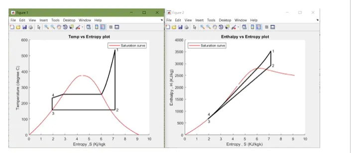
12. plt of t vs s and h vs s is create from all the point obtained from the program

13. the plot changes as the user input change for the above mentioned inputs.

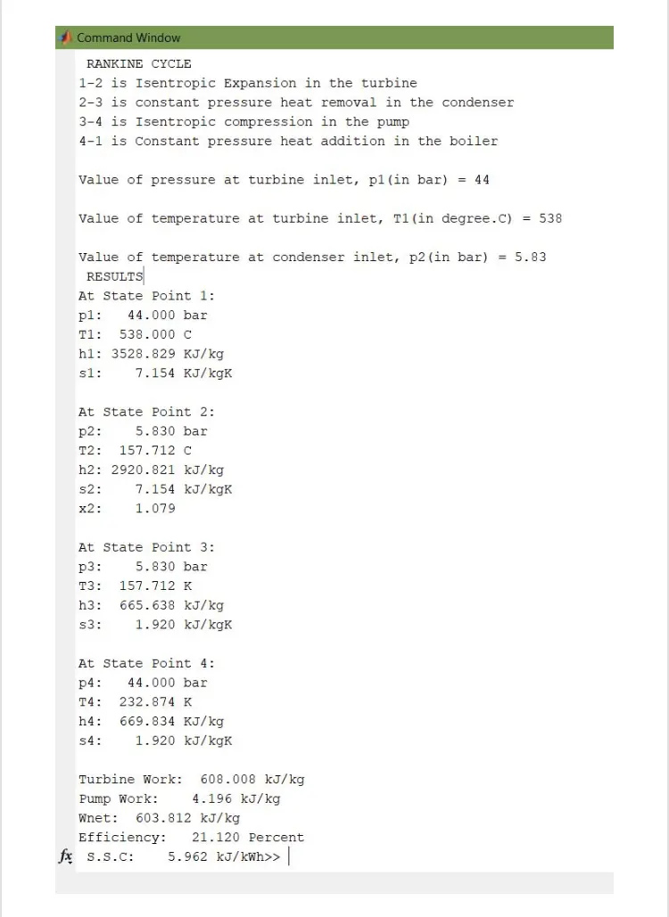
15. results are displyed in the command window.