Project 2 - Rankine cycle Simulator
% A Program to Rankine Cycle
clear all
close all
clc
%User Input
fprintf('%55s','Rankine Cycle Simulator')
fprintf('nn1 - 2 is Isentropic Expansion in the Turbine')
fprintf('n2 - 3 Constant Pressure Heat Rejection by the Condenser')
fprintf('n3 - 4 is Isentropic Compression in the Pump')
fprintf('n4 - 1 is Constant Pressure Heat Addition by the Boiler')
p1 = input('nnEnter the Pressure at the Turbine Inlet (in bar):n');
t1 = input('nEnter the Temperature at the Turbine Inlet (in Degree Celcius):n');
p2 = input('nEnter the Pressure at the Condenser Inlet (in bar):n');
%Turbine Inlet
s1 = XSteam('s_pT',p1,t1);
h1 = XSteam('h_pT',p1,t1);
%Condenser Inlet
s2 = s1;
sf2=XSteam('sL_p',p2);
sg2=XSteam('sV_p',p2);
hf2=XSteam('hL_p',p2);
hg2=XSteam('hV_p',p2);
%`Determining Dryness fraction`
if(s2 <= sg2)
x2 = ((s2 - sf2) / (sg2 - sf2));
else
x2 = 1;
end
h2 = hf2 + (x2 * (hg2 - hf2));
%Pump Inlet
p3 = p2;
t3 = XSteam('Tsat_p',p3);
s3 = XSteam('sL_p',p3);
h3 = XSteam('hL_p',p3);
t2 = t3;
%Boiler Inlet
p4 = p1;
s4 = s3;
h4 = XSteam('h_ps',p4,s4);
cp = XSteam('Cp_ps',p4,s4); %Isobaric specific heat
cv = XSteam('Cv_ps',p4,s4); %Isochoric specific heat
%Determining Gamma
gamma = ( cp / cv );
t4 = (t3 * (( p3 / p4 )^(( 1 - gamma) / gamma)));
%Work Done
%Work Done by the Turbine
Wt = h1 - h2;
%Work Done by the Pump
Wp = h4 - h3;
%Net Work Done
Wnet = Wt - Wp;
%Heat Added
%Heat Added in the Boiler
qin = h1 - h4;
%Heat Rejected in the Condensor
qout = h2 - h3;
%Thermal Efficiency
n = (Wnet / qin) * 100;
%Specific Steam Consumption
SSC = (3600/Wnet);
%Result
fprintf('%45s nnn','Result');
fprintf('%s %50s n','At State Point 1','At State Point 4');
fprintf('%s %.2f%s %40s %.2f%s n',' P1 is :',p1,' Bar',' P4 is :',p4,' Bar');
fprintf('%s %.2f%s %31s %.2f%s n',' T1 is :',t1,' Deg Celcius',' T4 is :',t4,' Deg Celcius');
fprintf('%s %.2f%s %36s %.2f%s n',' H1 is :',h1,' kJ/kg',' H4 is :',h4,' kJ/kg');
fprintf('%s %.2f%s %38s %.2f%s nn',' S1 is :',s1,' kJ/kgK',' S4 is :',s4,' kJ/kgK');
fprintf('%s %41s %.2f%s n','At State Point 2','Wt is :',Wt,' kJ/kg');
fprintf('%s %.2f%s %40s %.2f%s n',' P2 is :',p2,' Bar','Wp is :',Wp,' kJ/kg');
fprintf('%s %.2f%s %33s %.2f%s n',' T2 is :',t2,' Deg Celcius','Wnet is :',Wnet,' kJ/kg');
fprintf('%s %.2f%s %39s %.2f%s n',' H2 is :',h2,' kJ/kg','Ntherm is :',n,' Percent');
fprintf('%s %.2f%s %40s %.2f%s n',' S2 is :',s2,' kJ/kgK','S.S.C is :',SSC,' kg/kWh');
fprintf('%s %.2fnn','X2 is :',x2);
fprintf('%s n','At State Point 4');
fprintf('%s %.2f%s n',' P1 is :',p4,' Bar');
fprintf('%s %.2f%s n',' T1 is :',t4,' Deg Celcius');
fprintf('%s %.2f%s n',' H1 is :',h4,' kJ/kg');
fprintf('%s %.2f%s n',' S1 is :',s4,' kJ/kgK');
%Plotting
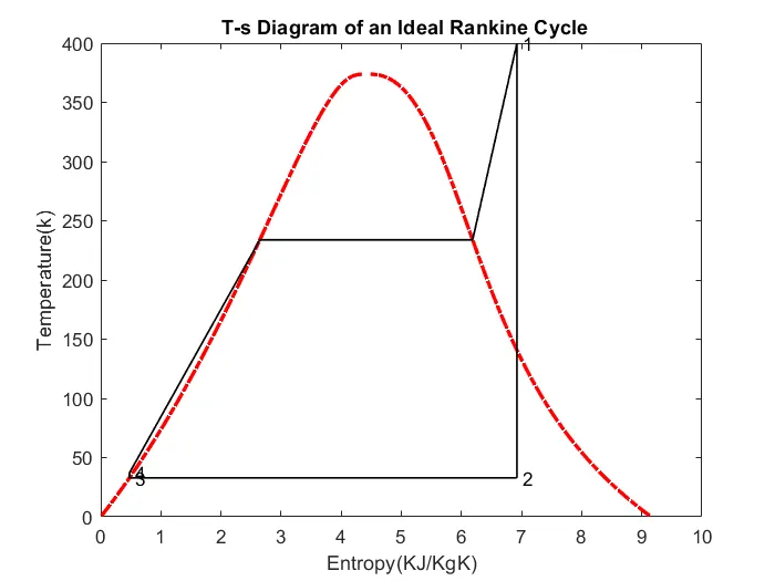
%TS Diagram
t = linspace(1,t1,2000);
for i = 1: 2000
sl(i) = XSteam('sL_T',t(i));
end
for i = 1: 2000
sv(i) = XSteam('sV_T',t(i));
end
figure(1)
plot(sl,t,'-.r','LineWidth',2)
hold on
plot(sv,t,'-.r','LineWidth',2)
title(' T-s Diagram of an Ideal Rankine Cycle')
xlabel('Entropy(KJ/KgK)')
ylabel('Temperature(k)')
%1-2 State
plot([s1 s2],[t1 t2],'k','LineWidth',1)
%2-3 State
plot([s2 s3],[t2 t3],'k','LineWidth',1)
%3-4 State
plot([s3 s4],[t3 t4],'k','LineWidth',1)
%4-1 State
tp = XSteam('TSat_p',p4);
sp = XSteam('sL_T',tp);
tq = tp;
sq = XSteam('sV_T',tq);
plot([s4,sp],[t4,tp],'k','LineWidth',1)
plot([sp sq],[tp tq],'k','LineWidth',1)
plot([sq,s1],[tq,t1],'k','LineWidth',1)
text(s1,t1,' 1');
text(s2,t2,' 2');
text(s3,t3,' 3');
text(s4,t4,' 4');
%PV Diagram
for i = 1: 2000
hl(i) = XSteam('hL_T',t(i));
end
for i = 1: 2000
hv(i) = XSteam('hV_T',t(i));
end
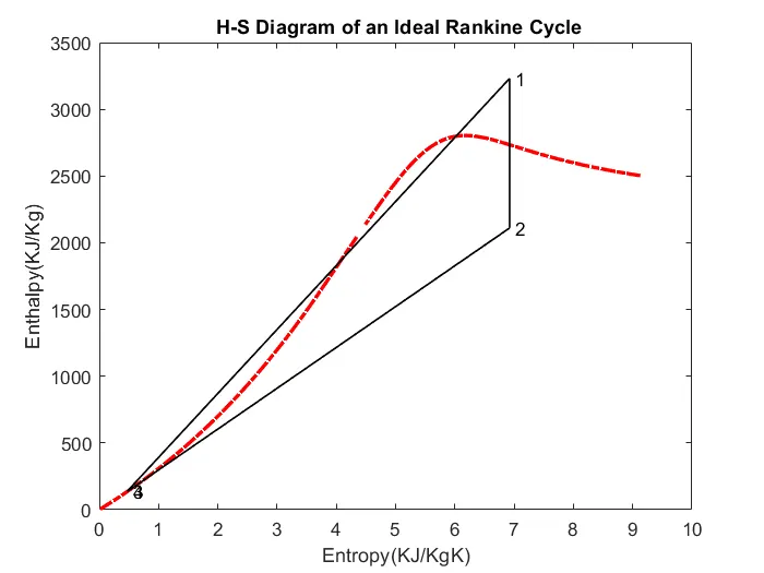
figure(2)
plot(sl,hl,'-.r','LineWidth',2)
hold on
plot(sv,hv,'-.r','LineWidth',2)
title(' H-S Diagram of an Ideal Rankine Cycle')
xlabel('Entropy(KJ/KgK)')
ylabel('Enthalpy(KJ/Kg)')
%1-2 State
plot([s1 s2],[h1 h2],'k','LineWidth',1)
%2-3 State
plot([s2 s3],[h2 h3],'k','LineWidth',1)
%3-4 State
plot([s3 s4],[h3 h4],'k','LineWidth',1)
%4-1 State
plot([s4 s1],[h4 h1],'k','LineWidth',1)
text(s1,h1,' 1');
text(s2,h2,' 2');
text(s3,h3,' 3');
text(s4,h4,' 4');
command windeo
Rankine Cycle Simulatornn
1 - 2 is Isentropic Expansion in the Turbinen
2 - 3 Constant Pressure Heat Rejection by the Condensern
3 - 4 is Isentropic Compression in the Pumpn
4 - 1 is Constant Pressure Heat Addition by the Boilernn
Enter the Pressure at the Turbine Inlet (in bar):n30
nEnter the Temperature at the Turbine Inlet (in Degree Celcius):n400
nEnter the Pressure at the Condenser Inlet (in bar):n0.05
Result
nnnAt State Point 1 At State Point 4 n P1 is : 30.00 Bar P4 is : 30.00 Bar n T1 is : 400.00 Deg Celcius T4 is : 36.94 Deg Celcius n H1 is : 3231.57 kJ/kg H4 is : 140.76 kJ/kg n S1 is : 6.92 kJ/kgK S4 is : 0.48 kJ/kgK nnAt State Point 2 Wt is : 1120.86 kJ/kg n P2 is : 0.05 Bar Wp is : 3.00 kJ/kg n T2 is : 32.88 Deg Celcius Wnet is : 1117.87 kJ/kg n H2 is : 2110.71 kJ/kg Ntherm is : 36.17 Percent n S2 is : 6.92 kJ/kgK S.S.C is : 3.22 kg/kWh nX2 is : 0.81nnAt State Point 4 n P1 is : 30.00 Bar n T1 is : 36.94 Deg Celcius n H1 is : 140.76 kJ/kg n S1 is : 0.48 kJ/kgK n>>