FINAL INDEPENDENT PROJECT

PROJECT TITLE: Braking systems

Aim: Ideal brake force repartition

Objective: The brake system takes the kinetic energy of your moving vehicle and converts it to thermal energy through friction. ... Usually used for the back wheels (although some vehicles had four-wheel drum brakes), drum brakes feature a hollow cylinder (the drum) attached to the axle that spins with the wheel

Electromagnetic

Electromagnetic brakes are likewise often used where an electric motor is already part of the machinery. For example, many hybrid gasoline/electric vehicles use the electric motor as a generator to charge electric batteries and also as a regenerative brake. Some diesel/electric railroad locomotives use the electric motors to generate electricity which is then sent to a resistor bank and dumped as heat. Some vehicles, such as some transit buses, do not already have an electric motor but use a secondary "retarder" brake that is effectively a generator with an internal short circuit. Related types of such a brake are eddy current brakes, and electro-mechanical brakes (which actually are magnetically driven friction brakes, but nowadays are often just called "electromagnetic brakes" as well).

Electromagnetic brakes slow an object through electromagnetic induction, which creates resistance and in turn either heat or electricity. Friction brakes apply pressure on two separate objects to slow the vehicle in a controlled manner.

Brake rotor convection

Study the temperature rise of a brake disc during a single stop and during continuous operation, simulating "N" identical braking maneuvers. There is also an estimation of the brake discs convection coefficient in terms of the vehicle speed, which could be useful to get a rough initial idea of its trend.

Brake load repartition

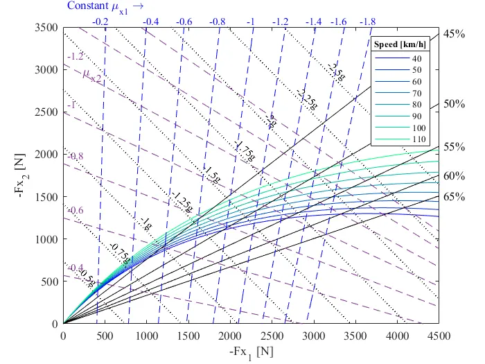
Evaluate the distribution of braking forces in the front and rear axle in ideal conditions, and compare with the system response, based on the vehicle data (mass, geometry, hydraulic system components)

Description:

FAD: Brake disc front
FPD: Brake disc rear
FPT: Rear brake drum
CF: Brake control
SF: servo brake
PF: Brake Pump
SLF: Brake Fluid Reservoir
RF: Splitter braking

FS: Parking Brake

Braking axle

clear all
close all

% Define symbols
syms Fx1 Fx2 b a l hcg m g Fzaerof Fzaeror mux F_drag;

%Ideal braking equations
(Fx1-Fx2)==mux*(m*g/l*(b-a+mux*2*hcg)+(Fzaerof-Fzaeror)-2*F_drag*hcg/l+2*mux*(Fzaerof+Fzaeror)*hcg/l);
mux=(Fx1+Fx2)/(m*g+Fzaerof+Fzaeror);

eqn=mux*(m*g/l*(b-a+mux*2*hcg)+(Fzaerof-Fzaeror)-2*F_drag*hcg/l+2*mux*(Fzaerof+Fzaeror)*hcg/l)-(Fx1-Fx2)

%Solve for the force in the rear axle
solve(eqn,Fx2)
%% Vehicle data
rho_air=1.16; %kg/m3
front_area=1; %m2
Cz_frontxS=1.504;
Cz_rearxS=1.696;
CxS=1.12;
m=275; %kg
g=9.81; %m/s^2
l= 1.525; a=0.808; b=l-a; hcg=0.245; %m

%% Brake system parameters
%This section contains all the functional parameters of the brake system.
%The parameter values can be modified to evaluate different configurations.

%Pedal Box
Pedal_ratio=3.03 %Brake pedal mechanical advantage
Preload=0; %Spring preload [N]
fMC_Diam=19 %Front master cylinder piston diameter[mm]
rMC_Diam=16 %Rear master cylinder piston diameter[mm]
AMCf=pi*fMC_Diam^2/4 % Section area of front MC mm^2
AMCr=pi*rMC_Diam^2/4 % Section area of rear MC mm^2

%Brake Calipers
fCaliper_diam=24 %Front calipers piston diameter[mm]
fCaliper_PistonQty=4
ACf=pi*fCaliper_diam^2/4*fCaliper_PistonQty % Front caliper pistons area mm^2
rCaliper_diam=24 %Rear calipers piston diameter[mm]
rCaliper_PistonQty=2
ACr=pi*rCaliper_diam^2/4*rCaliper_PistonQty % Rear caliper pistons area mm^2

frpad=94 %front caliper effective radius
rrpad=83 %Rear caliper effective radius

%% Solve the symbolic equations for different values of initial speed
n=45
j=1;
v=linspace(40/3.6,110/3.6,8);

for V= v

F_drag(j)=0.5*rho_air*front_area*CxS*V^2; %[N]
Fz_aero_front=0.5*rho_air*front_area*Cz_frontxS*V^2; %[N]
Fz_aero_rear=0.5*rho_air*front_area*Cz_rearxS*V^2;
Fzaerof=Fz_aero_front; Fzaeror=Fz_aero_rear;
syms Fx1 Fx2
mux=(Fx1+Fx2)/(m*g+Fzaerof+Fzaeror);

eqn=mux*(m*g/l*(b-a+mux*2*hcg)+(Fzaerof-Fzaeror)-2*F_drag(j)*hcg/l+...
2*mux*(Fzaerof+Fzaeror)*hcg/l)-(Fx1-Fx2);
Fx1_it=0;

for i=1:n
Fx1=Fx1_it;
RATIO=subs(eqn);
SolFx2=solve(RATIO,Fx2,'real',true); %'ReturnConditions',true
Fx2_calc(i)=double(SolFx2(2));
g_decel(j,i)=(Fx1_it+Fx2_calc(i)-F_drag(j))/(m*g);
% plot(Fx1_input,g_decel')
Fx1_it=Fx1_it+100;
end

FX2(j,:)=Fx2_calc;
j=j+1;

end

Fx1_input=linspace(0,Fx1_it,n);
[numRows,numCols] = size(FX2);

%% Plot the ideal brake force repartition curves at different speeds

% Define Colormap for Force lines
cm = colormap(winter(numRows));
for i=1:length(v)
f(i)=plot(Fx1_input,FX2(i,:),'Color', cm(i,:));
hold on
end
GRAPH=gcf;
set(gca, 'FontName', 'Times')
xlabel('-Fx_1 [N]'),ylabel('-Fx_2 [N]')
hold on

graph = gca;

%% Add lines with system response at different balance bar setups

%Create hidden axes for adding the bias labels outside
bias_labels=axes('Position',[0 0 1 1],'Visible','off');
set(gcf,'CurrentAxes',graph)
bar_ratio=linspace(0.45/0.55,0.65/0.35,5)
front_bias=linspace(0.45,0.65,length(bar_ratio))
cm2 = colormap(hot(length(bar_ratio)+2));
for k=1:length(bar_ratio)
Tqratio=bar_ratio(k)*(AMCr*frpad*ACf)/(AMCf*rrpad*ACr);
Fx2_real=Fx1_input/Tqratio;
set(gcf,'CurrentAxes',graph)
f(i+k)=plot(Fx1_input,Fx2_real,'Color','k','LineWidth',.3);
text(max(Fx1_input)+50,max(Fx2_real),num2str(100*(front_bias(k)),'%g%%'),'FontName','Times','FontSize',10)
end

% Fix the axes limits
ymax=([0 3500]); ylim(ymax) %define maximum Y limits for the plot
xmax=([0 4500]); xlim(xmax) %define maximum x limits for the plot
positionax=[200 650 0]; %Initial position for the constant deceleration tags

%% Add lines with constant longitudinal decelerations
ax=linspace(0.5,2.5,9);
for iax=1:length(ax)
FX2ax=-Fx1_input+m*ax(iax)*9.81-double(F_drag(8));
Const_ax(iax)=plot(Fx1_input,FX2ax,'k:','LineWidth',1)
t=text(positionax(1)+(iax-1)*290*xmax(2)/ymax(2),positionax(2)+(iax-1)*390*ymax(2)/xmax(2),{[num2str(-ax(iax),3) 'g']},'Rotation',-atan(ymax(2)/xmax(2))*180/pi-5,'FontSize',9,'FontName','Times')
end

%% Add lines with constant friction coefficients and labels

%Front axle friction coefficient
ux1=linspace(0.2,1.8,9);
for iux1=1:length(ux1)
FX2ux1=-Fx1_input*(l/(ux1(iux1)*hcg)+1)+m*g*b/hcg+0.5*rho_air*Cz_frontxS*l/hcg*v(8)^2;
Const_ux1(iux1)=plot(Fx1_input,-FX2ux1,'b--','LineWidth',.3)
hold on
end

%Add labels
text(50,ymax(2)+240,'Constant \mu_x_1 \rightarrow ','FontSize',10,'FontName','Times','Color','b')
text(350,ymax(2)+75,{num2str(-ux1(1),2)},'Rotation',0,'FontSize',9,'FontName','Times','Color','b')
text(950,ymax(2)+75,{num2str(-ux1(2),2)},'Rotation',0,'FontSize',9,'FontName','Times','Color','b')
text(1350,ymax(2)+75,{num2str(-ux1(3),2)},'Rotation',0,'FontSize',9,'FontName','Times','Color','b')
text(1750,ymax(2)+75,{num2str(-ux1(4),2)},'Rotation',0,'FontSize',9,'FontName','Times','Color','b')
text(2200,ymax(2)+75,{num2str(-ux1(5),2)},'Rotation',0,'FontSize',9,'FontName','Times','Color','b')
text(2500,ymax(2)+75,{num2str(-ux1(6),2)},'Rotation',0,'FontSize',9,'FontName','Times','Color','b')
text(2900,ymax(2)+75,{num2str(-ux1(7),2)},'Rotation',0,'FontSize',9,'FontName','Times','Color','b')
text(3200,ymax(2)+75,{num2str(-ux1(8),2)},'Rotation',0,'FontSize',9,'FontName','Times','Color','b')
text(3550,ymax(2)+75,{num2str(-ux1(9),2)},'Rotation',0,'FontSize',9,'FontName','Times','Color','b')

%Rear axle friction coefficient
ux2=linspace(0.4,1.6,7);
cm3 = colormap(winter(length(ux2)+2));
for iux2=1:length(ux2)
FX2ux2=-Fx1_input*(ux2(iux2)*a)/(-l-ux2(iux2)*hcg)+(ux2(iux2)*m*g*a)/(l+ux2(iux2)*hcg)-(0.5*rho_air*Cz_rearxS*v(8)^2*l)/(ux2(iux2)*hcg+l);
Const_ux2(iux2)=plot(Fx1_input,flip(FX2ux2),'--','LineWidth',.3,'Color',[0.4940 0.1840 0.5560])%[0.4660, 0.6740, 0.1880])
hold on
if iux2<=5
text(50,max(FX2ux2)+100,{ num2str(-ux2(iux2),2)},'FontSize',9,'FontName','Times','Color',[0.4940 0.1840 0.5560])
end
end

text(230,ymax(2)-550,'\mu_x_2','Rotation',0,'FontSize',11,'FontName','Times','Color',[0.4940 0.1840 0.5560])

% %% Include the bias valve working region
%
% valve=[500 1300]
% Tqratio=0.4/0.60*(AMCr*frpad*ACf)/(AMCf*rrpad*ACr);
% for k=1:length(valve)
% for i=1:length(Fx1_input)
% if Fx1_input(i)<=valve(k)
% Fx2_bias(k,i)=Fx1_input(i)/Tqratio;
% elseif Fx1_input(i)>valve(k) && k==1
% Fx2_bias(k,i)= Fx1_input(min(find(Fx1_input>valve(k))))/Tqratio+Fx1_input(i)*0.325-88.4+137-274.1+20;
% elseif Fx1_input(i)>valve(k) && k==2
% Fx2_bias(k,i)= Fx1_input(min(find(Fx1_input>valve(k))))/Tqratio+Fx1_input(i)*0.325-284-480+60+10+57+15+108+15+37.9+20;
%
% end
% end
%
% hold on
% BIAS=plot(Fx1_input,Fx2_bias,'Color','y','LineWidth',.3);
% %
% end
%
% % Fill region of operation
% x2 = [Fx1_input, fliplr(Fx1_input)];
% inBetween = [Fx2_bias(1,:), fliplr(Fx2_bias(2,:))];
% h=fill(x2, inBetween, 'y');
% set(h,'facealpha',.1)

%% Final formatting
leg1=legend(f(1:length(v)),'40 ','50','60','70','80','90','100','110','Location','northeast','FontSize',8);
title1 = get(leg1,'Title'); set(title1,'String',{'Speed [km/h]'});