Project 2 - Rankine cycle Simulator

Rankine cycle Simulator

Aim: Create a Rankine simulator using MATLAB.

Objectives:

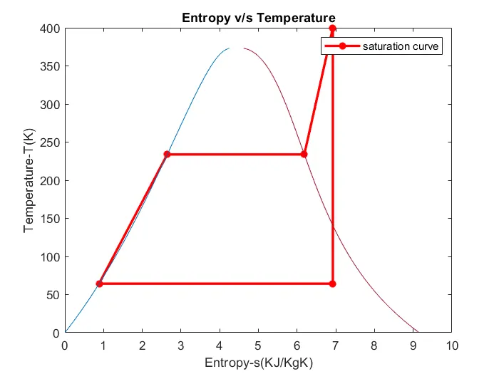
1. Graph of Entropy vs Temperature

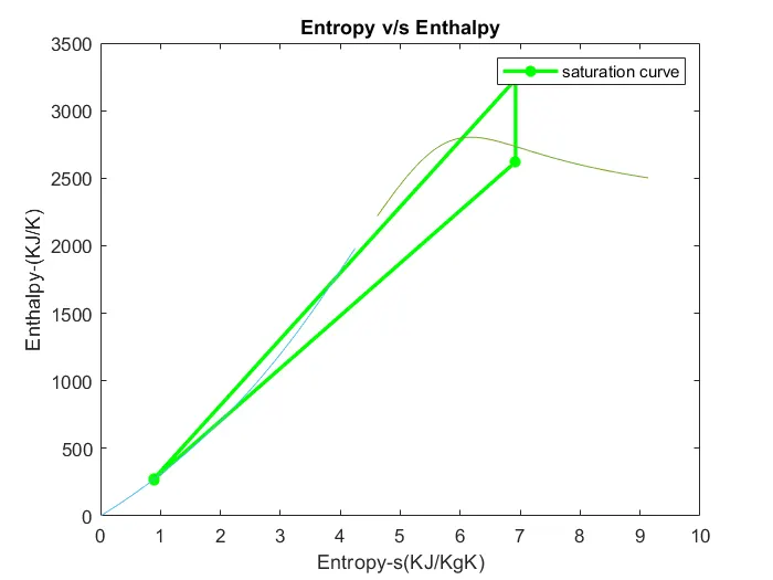
2. Graph of Entropy vs Enthalpy

Theory:

Rankine cycle

The Rankine cycle closely describes the process by which steam engines commonly found in thermal power generation plants harness the thermal energy of a fuel or other heat source to generate electricity. Possible heat sources include the combustion of fossil fuels such as coal, natural gas, or oil, renewable fuels like biomass or ethanol, nuclear fission, and concentrated solar power plant. Common heat sinks include ambient air above or around a facility and bodies of water such as rivers, ponds, and oceans.

The ability of a Rankine engine to harness energy depends on the relative temperature difference between the heat source and heat sink. The greater the differential, the more mechanical power can be efficiently extracted out of heat energy, as per Carnot's theorem.

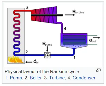
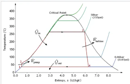
Process1-2: Isentropic compression.

Process2-3: Constant pressure heat addition.

Process3-4: Isentropic expansion.

Process4-1: Constant pressure heat rejection.

Governing equations:

`T_2/T_1 =(〖P_2/P_1 )〗^(1-(1/γ))`

T-Temperature (K).

P-Pressure(bar)

γ -Heat capacity ratio.

Net work,W_net=W_t-W_p

〖Bw〗_ratio=W_p/W_t

W_t=h1-h2

W_p=h4-h3

h – enthalpy (KJ/kg)

W_t – Turbine work (KJ/kg)

W_p- pump work (KJ/kg)

Procedure:

• clear all,close all, clc to erase the workspace and plots.
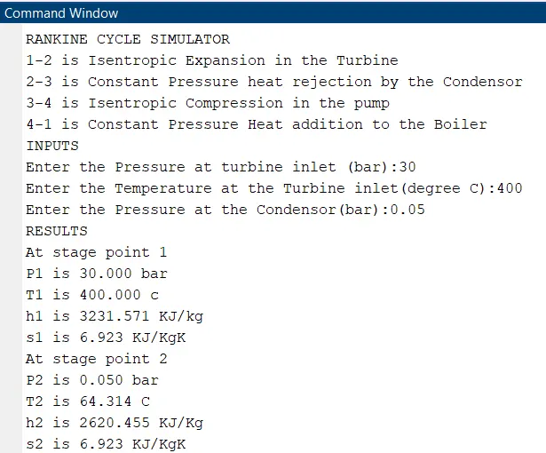
• input variables P1, P2, T1 are given by the input command whose values are entered in the command window while executing the program.
• state 1, values for enthalpy and entropy are extracted as a function of pressure and temperature.
• h_pT, s_pT, hL_p,sV_p are the default variable whose value is stored in XSteam.
• Pressure, temperature, enthalpy, entropy for all the state variables are extracted as a function of the dependent variable from the XSteam file.
• Find pressure, temperature, enthalpy, entropy for each state point.
• finally work done, the heat evolved and SSE is calculated by basic formulae.
• To plot the saturation curve , the temperature range is defined using the linspace command and for the overall length of this temperature values of enthalpy and entropy are calculated at every temperature point. The break in the saturation curve separates the liquid phase and vapor phase .
• Plotting both T-S and H-S curves using the plot commands.
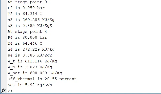
• Results of the cycle simulations are displayed over the command window by putting the required inputs.

Error:

1.

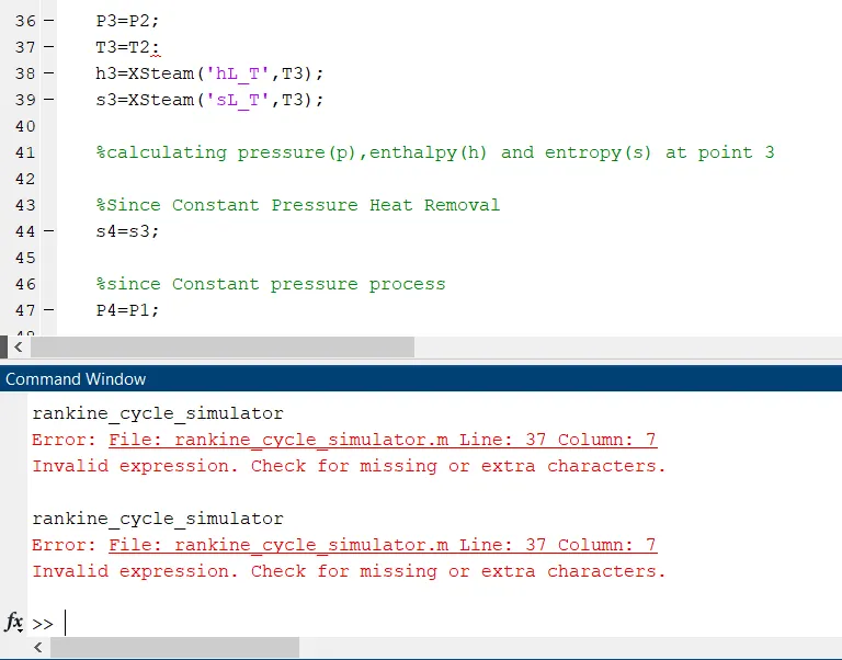
Syntax error-put colon instead of a semicolon.

Conclusion:

Created a Rankine simulator using MATLAB.

Output screen-