Project 2 - Rankine cycle Simulator

Rankine Cycle - It is an idealized thermodynamic cycle where heat is converted into mechanical work with change in phase and without considering th friction losses.

It has four stages

Isentropic Expansion (Turbine)

Constant Pressure Heat Rejection (Condenser)

Isentropic Compression (Pump)

Constant Pressure Heat Addition (Boiler)

Code

close all
clear all
clc

%Printing Descriptions
fprintf('Rankine Cycle Simulator\n')
fprintf('1-2 Isobaric Heat Addition\n')
fprintf('2-3 Isentropic Expansion\n')
fprintf('3-4 1-2 Isobaric Heat Rejection\n')
fprintf('4-1 Isentropic Compression\n')

%Enter The Input Parameters
p1 = input(' Enter Pressure at Turbine inlet (bar):');
T1 = input(' Enter Temperature at Turbine inlet (Celsius):');
p2 = input(' Enter Pressure at Condenser (bar):');

%calculation of state point values
%state point 1
h1 = XSteam('h_pt',p1,T1);
s1 = XSteam('s_pt',p1,T1);

%state point 2
s2=s1;
sf2 = XSteam('sL_p',p2);
sg2 = XSteam('sV_p',p2);
hf2 = XSteam('hL_p',p2);
hg2 = XSteam('hV_p',p2);
s2 = sg2;
h2 = hg2;
T2 = XSteam('T_hs',h2,s2);

%state point 3
T3 = T2;
p3 = p2;
s3 = XSteam('sL_T',T3);
h3 = XSteam('hL_T',T3);
v3 = XSteam('vL_p',p2);

%state point 4
p4=p1;
s4=s3;
Cp4 = XSteam('Cp_ps',p4,s4);
Cv4 = XSteam('Cv_ps',p4,s4);
gamma = Cp4/Cv4;
r = (gamma - 1)/gamma;
T4 = T3*(p4/p3)^r;

%Calculating other output values
Wt = h1 - h2; %Turbine Output
Wp = v3*(p1-p2)*100; %Pump output
h4 = Wp + h3;
Wnet = Wt - Wp;  %NetWork in KJ/Kg
Qs = h1 - h4;
N_per = (Wnet/Qs)*100; %Efficiency
Steam_rate = 3600/Wnet;

%state point 5 and 6
T5 = XSteam('Tsat_p',p1);
T6 = T5;
s5 = XSteam('sL_p',p1);
s6 = XSteam('sV_p',p1);
h5 = XSteam('hL_p',p1);
h6 = XSteam('hV_p',p1);

fprintf('\n RESULTS \n')
fprintf('At State Point 1: \nP1 is : %4.2f Bar\nT1 is : %4.2f Celsius\nH1 is : %4.2f KJ/Kg\nS1 is : %4.2f KJ/KgK\n\n', p1,T1,h1,s1)
fprintf('At State Point 2: \nP1 is : %4.2f Bar\nT2 is : %4.2f Celsius\nH2 is : %4.2f KJ/Kg\nS2 is : %4.2f KJ/KgK\n\n', p2,T2,h2,s2)
fprintf('At State Point 3: \nP1 is : %4.2f Bar\nT3 is : %4.2f Celsius\nH3 is : %4.2f KJ/Kg\nS3 is : %4.2f KJ/KgK\n\n', p3,T3,h3,s3)
fprintf('At State Point 4: \nP1 is : %4.2f Bar\nT4 is : %4.2f Celsius\nH4 is : %4.2f KJ/Kg\nS4 is : %4.2f KJ/KgK\n\n', p4,T4,h4,s4)

%plotting 
subplot(1,2,1)
T_rankine = linspace(T5,T1,5000);
for i= 1:length(T_rankine)
    s_rankine(i) =  XSteam('s_pT',p1,T_rankine(i));
end
plot([s1 s2 s3 s4 s5 s6 s_rankine],[T1 T2 T3 T4 T5 T6 T_rankine],'linewidth',1.5);
hold on
T_curve = linspace(1,400,500);
for i =1:length(T_curve)
    s_l(i) = XSteam('sL_T',T_curve(i));
    s_v(i) = XSteam('sV_T',T_curve(i));
    h_l(i) = XSteam('hL_T',T_curve(i));
    h_v(i) = XSteam('hV_T',T_curve(i));
end
%plot T-S diagram
plot(s_l,T_curve);
plot(s_v,T_curve);
text(s1,T1,'1')
text(s2,T2,'2')
text(s3,T3,'3','HorizontalAlignment','right','VerticalAlignment','top')
text(s4,T4,'4','HorizontalAlignment','right','VerticalAlignment','bottom')
text(s5,T5,'5')
text(s6,T6,'6')
xlabel('Entropy (KJ/KgK)');
ylabel('Temperature (Celcius)');

%plot H-S diagram
subplot(1,2,2)
plot([s1 s2 s3 s4 s1],[h1 h2 h3 h4 h1],'linewidth',2);
hold on
plot(s_v,h_v)
plot(s_l,h_l)
text(s1,h1,'1')
text(s2,h2,'2')
text(s3,h3,'3','HorizontalAlignment','right','VerticalAlignment','top')
text(s4,h4,'4','HorizontalAlignment','right','VerticalAlignment','bottom')
xlabel('Entropy (KJ/KgK)');
ylabel('Enthalpy (KJ/Kg)');

Output in Command Window

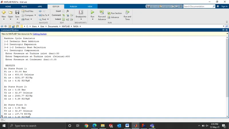
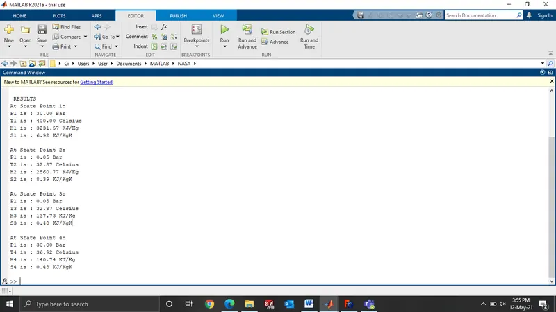
Workspace

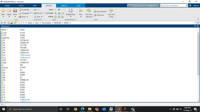
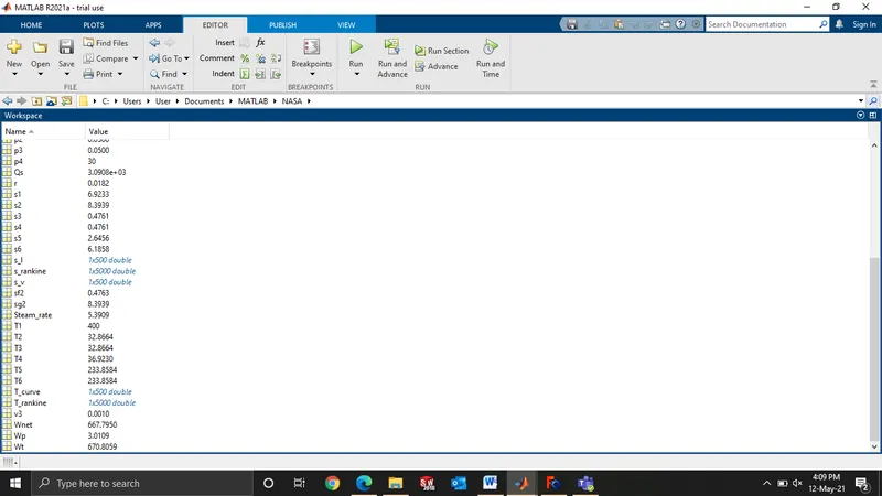
Error

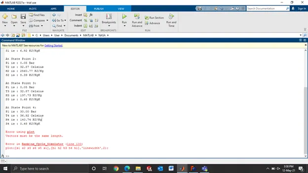
There was a typing mistake and s5 was added, later on removing it the program ran smoothly

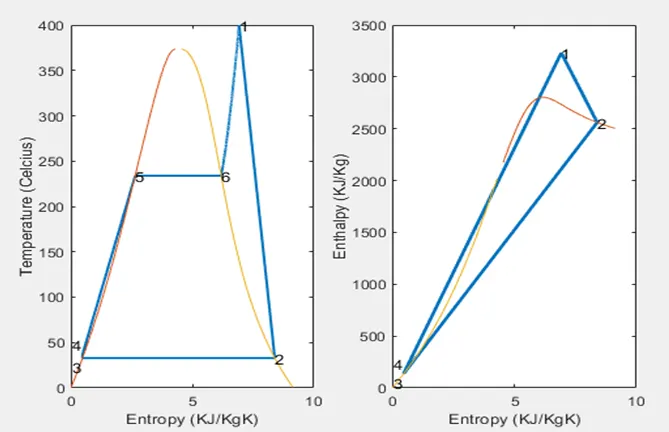
Plots

Code Explanation -

- Input is taken for pressure at points 1 and 2 and for tempertaure at point 1.

- State 1 values of enthalpy and entropy are extracted as a fucntion of temperature and pressure.

- some of the default variables are stored in the XSteam file and are called s_pT, h_pT etc.

- All the state variable for temperature, pressure, entropy and enthalphy are extracted.

- two more points 5 and  6 are plotted to complete the cycle.

- Heat ejected, work done and SSC are calculated from the basic formulae.

- The Vapour dome is plotted useing the length of the overall temperature values. The break in saturation curve seperates the Liquid and Vapour phase.

- After retrieving all the data T-s and H-s curves are plotted.