Project 2 - Rankine cycle Simulator
Objective:
- To create a Rankine cycle (Ideal Rankine cycle) simulator using MATLAB.
- To evaluate state points and plot T-s and h-s graph for the cycle.
Description:
The Rankine cycle is a model used to predict the performance of steam turbine systems. It was also used to study the performance of reciprocating steam engines. The Rankine cycle is an idealized thermodynamic cycle of a heat engine that converts heat into mechanical work while undergoing phase change.
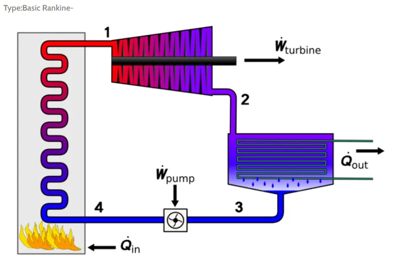
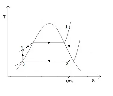
The Rankine cycle is the ideal cycle for vapor power plants; it includes the following four reversible processes:
- Process 4-1: Reversible constant pressure heating of water (Q1) in boiler
- Process 1-2: Reversible adiabatic expansion of steam in turbine (Wt)
- Process 2-3: Reversible constant pressure heat rejection (Q2) in condenser
- Process 3-4: Reversible adiabatic input work (Wp) in pump
For 1kg of fluid, the steady flow energy equation to each processes:
- For boiler Q1 = h1-h4
- For turbine Wt = h1-h2
- For condenser Q2 = h2-h3
- For pump Wp = h4-h3
- Efficiency, Eta = Wnet/Q1 = {(h1-h2)-(h4-h3)}/ (h1-h4)
- Work ratio (WR) = (Wt-Wp)/ Wt
- Back work ratio BWR = Wp/Wt
In general, pump work is very small as compared to turbine work so often neglected. Only sensible heat will be extracted by condenser.
Terms used:
- Enthalpy (Specific Enthalpy) : Specific Enthalpy is the total energy in a system due to pressure and temperature per unit of mass in that system.
- Entropy (Specific Entropy) : Specific Entropy is entropy per unit mass. Entropy, the measure of a system's thermal energy per unit temperature that is unavailable for doing useful work.
Saturation curve:
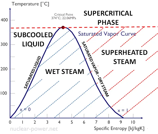
- A saturation state is the point where a phase change begins or ends.
- The saturation vapor curve is the curve separating the two-phase state and the superheated vapor state in the T–s diagram.
- The saturated liquid curve is the curve separating the subcooled liquid state and the two-phase state in the T–s diagram.
- Saturation temperature means boiling point. The saturation temperature is the temperature for a corresponding saturation pressure at which a liquid boils into its vapor phase.
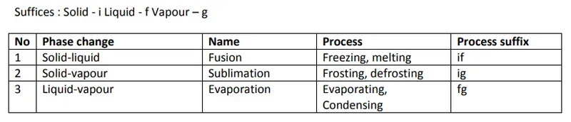
- phase change terminology
- Dryness fraction (x) is related with wet steam. It is defined as the ratio of the mass of actual dry steam to the mass of steam containing it.
- Sensible heat of water (hf) is the quantity of heat absorbed by 1 kg of water when it is heated from 0°C (freezing point) to boiling point.
- Latent heat or hidden heat (hfg) is the amount of heat required to convert water at a given temperature and pressure into steam at the same temperature and pressure.
- Enthalpy of wet steam (h) is defined as the quantity of heat required to convert 1 kg of water at 0°C into wet steam at constant pressure. It is the sum of total heat of water and the latent heat and this sum is also called enthalpy. In other words, h = hf + xhfg
- When steam is heated after it has become dry and saturated, it is called superheated steam and the process of heating is called superheating. Superheating is always carried out at constant pressure.
- hf = Enthalpy of saturated liquid (kJ/kg)
- hfg = Enthalpy or latent heat of vapourisation (kJ/kg)
- hg = Enthalpy of saturated vapour (steam) (kJ/kg)
- sf = Entropy of saturated liquid (kJ/kg K)
- sfg = Entropy of vapourisation (kJ/kg K)
- sg = Entropy of saturated vapour (steam) (kJ/kg K)
- hfg = hg – hf .....Change of enthalpy during evaporation
- sfg = sg – sf .....Change of entropy during evaporation
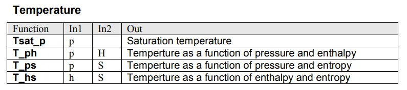
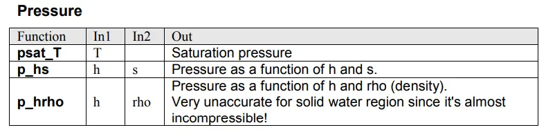
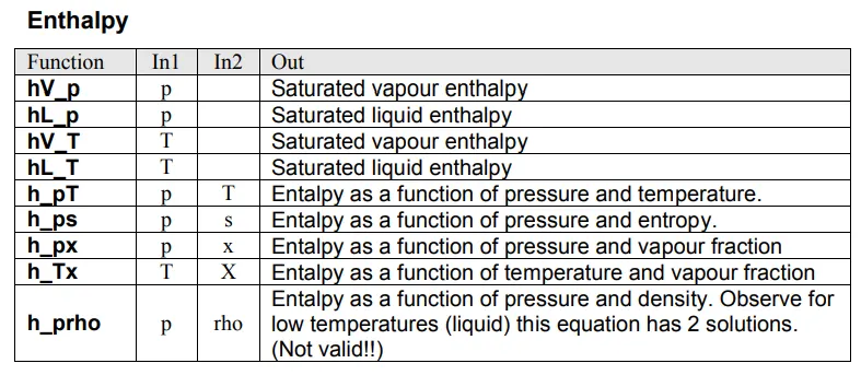
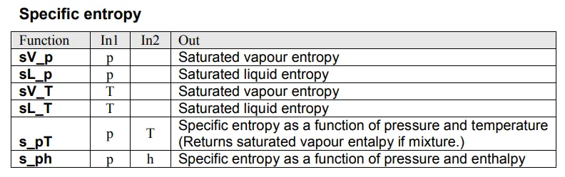
XSteam Library: X Steam for Matlab is a implementation of the IAPWS IF97 standard formulation. It provides accurate data for water and steam and mixtures of water and steam properties from 0 - 1000 bar and from 0 - 2000 deg C.
XSteam calling functions:
MATLAB code:
clear all
close all
clc

disp('_______________Rankine Cycle simulation_______________')
disp('1-2 Reversible adiabatic expansion of steam in turbine')
disp('2-3 Reversible constant pressure heat rejection in condenser')
disp('3-4 Reversible adiabatic input work in pump')
disp('4-1 Reversible constant pressure heating of water in boiler \n')

%Inputs:
disp('_______________ENTER INPUTS_______________');
p1 = input('Pressure at turbine inlet(bar):');
T1 = input('Temperature at Turbine inlet(degree C):');
p2 = input('Pressure at inlet of the condensor(bar):');

%Extracting and calculating State points
%state 1
h1 = XSteam('h_pT',p1,T1);
s1 = XSteam('s_ph',p1,h1);

%state 2
s2 = s1;
T2 = XSteam('T_ps',p2,s2);
sf2 = XSteam('sL_p',p2);
sg2 = XSteam('sV_p',p2);
sfg2 = sg2-sf2;
x2 = (s2-sf2)/sfg2;
hf2 = XSteam('hL_p',p2);
hg2 = XSteam('hV_p',p2);
hfg2 = hg2-hf2;
h2 = hf2+(x2*hfg2);

%state 3
p3 = p2;
T3 = T2;
s3 = XSteam('sL_p',p3);
h3 = XSteam('hL_p',p3);

%state 4
s4 = s3;
p4 = p1;
T4 = XSteam('T_ps',p4,s4);
h4 = XSteam('h_pT',p4,T4);

%Heat supplied for boiler
Q1 = h1-h4;

%Heat rejected from condenser
Q2 = h2-h3;

%Work done by turbine
Wt = h1-h2;

%Work done on pump
Wp = h4-h3;

%Net work
Wnet = Wt-Wp;

%Efficiency of Ideal Rankine cycle (in percentage)
Efficiency = (Wnet/Q1)*100;

%Specific steam consumption or steam rate
SSC = 3600/Wnet;

%Back work ratio
BWR = Wp/Wt;

%Plotting the saturation curve
T = linspace(1,500,1000);
for i = 1:length(T)
sf(i) = XSteam('sL_T',T(i));
sg(i) = XSteam('sV_T',T(i));
hf(i) = XSteam('hL_T',T(i));
hg(i) = XSteam('hV_T',T(i));
end

%Plotting T-s diagram
figure(1)
hold on
plot(sf,T,'r','linewidth',0.5)
plot(sg,T,'r','linewidth',0.5)
plot([s1 s2],[T1 T2],'marker','*','color','b','linewidth',1)
plot([s2 s3],[T2 T3],'marker','*','color','b','linewidth',1)
plot([s3 s4],[T3 T4],'marker','*','color','b','linewidth',1)
s_entropy = linspace(s4,s1,3000);
for n = 1:length(s_entropy)
 T_temp(n) = XSteam('T_ps',p1,s_entropy(n));
end
plot(s_entropy,T_temp,'b','linewidth',1)

text(s1+0.1,T1,'1')
text(s2+0.1,T2,'2')
text(s3-0.1,T3-15,'3')
text(s4-0.1,T4+15,'4')
title('Temperature vs Entropy plot for RANKINE CYCLE')
xlabel('Entropy s (KJ/kgK)')
ylabel('Temperature (degree C)')
legend('Saturation curve','location','northeast')

%Plotting h-s diagram
figure(2)
hold on
plot(sf,hf,'r','linewidth',0.5)
plot(sg,hg,'r','linewidth',0.5)
plot([s1 s2],[h1 h2],'marker','*','color','b','linewidth',1)
plot([s2 s3],[h2 h3],'marker','*','color','b','linewidth',1)
plot([s3 s4],[h3 h4],'marker','*','color','b','linewidth',1)
plot([s4 s1],[h4 h1],'b','linewidth',1)

text(s1+0.1,h1,'1')
text(s2+0.1,h2,'2')
text(s3-0.1,h3-80,'3')
text(s4-0.1,h4+80,'4')
title('Enthalpy vs Entropy plot for RANKINE CYCLE')
xlabel('Entropy s (KJ/kgK)')
ylabel('Enthalpy h (KJ/kg)')
legend('Saturation curve','location','northeast')

% Displaying Results
disp('_______________RESULTS_______________');
fprintf('At State Point 1: \n');
fprintf('p1 is %10.3f bar \n',p1);
fprintf('T1 is %10.3f C \n',T1);
fprintf('h1 is %10.3f KJ/kg \n',h1);
fprintf('s1 is %10.3f KJ/kgK \n\n',s1);
fprintf('At State Point 2: \n');
fprintf('p2 is %10.3f bar \n',p2);
fprintf('T2 is %10.3f C \n',T2);
fprintf('h2 is %10.3f kJ/kg \n',h2);
fprintf('s2 is %10.3f kJ/kgK \n',s2);
fprintf('x2 is %10.3f \n\n',x2);
fprintf('At State Point 3: \n');
fprintf('p3 is %10.3f bar \n',p3);
fprintf('T3 is %10.3f K \n',T3);
fprintf('h3 is %10.3f kJ/kg \n',h3);
fprintf('s3 is %10.3f kJ/kgK \n\n',s3);
fprintf('At State Point 4: \n');
fprintf('p4 is %10.3f bar \n',p4);
fprintf('T4 is %10.3f K \n',T4);
fprintf('h4 is %10.3f KJ/kg \n',h4);
fprintf('s4 is %10.3f kJ/kgK \n\n',s4);
fprintf('Turbine Work: %8.3f kJ/kg \n',Wt);
fprintf('Pump Work: %11.3f kJ/kg \n',Wp);
fprintf('Wnet: %16.3f kJ/kg \n',Wnet);
fprintf('Efficiency: %10.3f Percent \n',Efficiency);
fprintf('Steam rate: %10.3f kg/kWh \n',SSC);
fprintf('Back work ratio: %1.3f \n',BWR);
Code explanation:
- Display command for introduction of Rankine cycle proceses at Command window is used initially.
- By using Input command, end-user will now have flexibility of assigning values of his choice/requirement.
- Values at state points are found by calling XSteam library function with proper syntax.
- 'for loop' and 'plot' commands are used to plot Saturation curve, T-s & h-s curves.
- 'fprintf' command is used to print all state properties values in command window.
Inputs given:
- Turbine Inlet Temperature = 400 degree C
- Turbine Inlet Pressure = 30 bar
- Turbine Outlet Pressure = 0.05 bar = Condenser Inlet Pressure
Command window result:
_______________Rankine Cycle simulation_______________
1-2 Reversible adiabatic expansion of steam in turbine
2-3 Reversible constant pressure heat rejection in condenser
3-4 Reversible adiabatic input work in pump
4-1 Reversible constant pressure heating of water in boiler \n
_______________ENTER INPUTS_______________
Pressure at turbine inlet(bar):30
Temperature at Turbine inlet(degree C):400
Pressure at inlet of the condensor(bar):0.05
_______________RESULTS_______________
At State Point 1:
p1 is     30.000 bar
T1 is    400.000 C
h1 is   3231.571 KJ/kg
s1 is      6.923 KJ/kgK

At State Point 2:
p2 is      0.050 bar
T2 is     32.875 C
h2 is   2110.708 kJ/kg
s2 is      6.923 kJ/kgK
x2 is      0.814

At State Point 3:
p3 is      0.050 bar
T3 is     32.875 K
h3 is    137.765 kJ/kg
s3 is      0.476 kJ/kgK

At State Point 4:
p4 is     30.000 bar
T4 is     32.945 K
h4 is    140.762 KJ/kg
s4 is      0.476 kJ/kgK

Turbine Work: 1120.863 kJ/kg
Pump Work:       2.997 kJ/kg
Wnet:         1117.865 kJ/kg
Efficiency:     36.167 Percent
Steam rate:      3.220 kg/kWh
Back work ratio: 0.003 Plots:
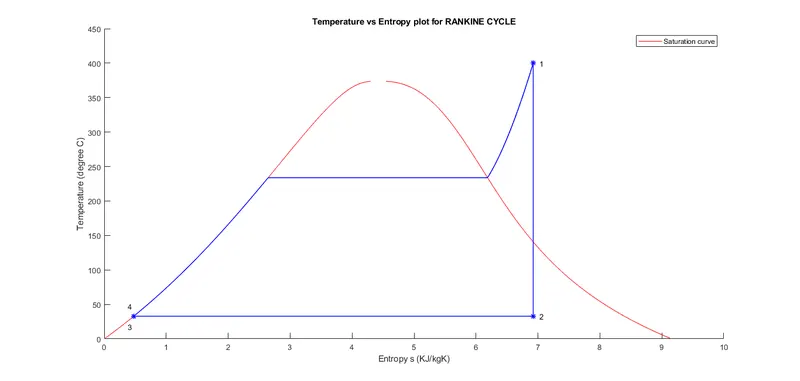
-
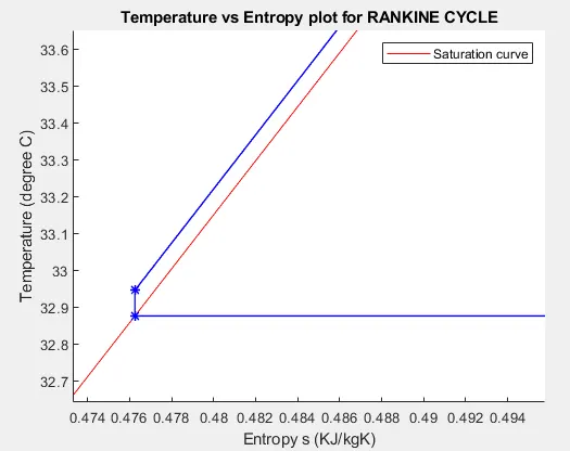 Zoom view of state points 3&4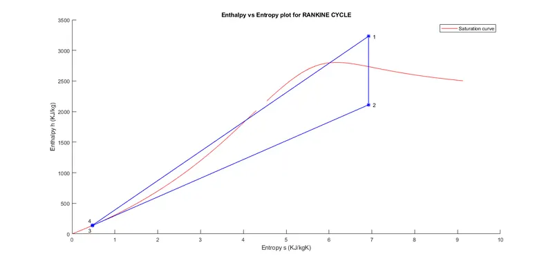
-
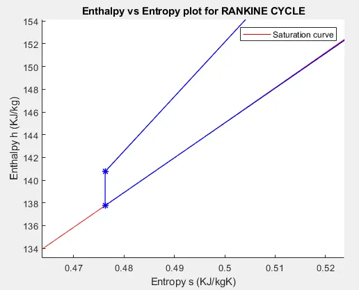 Zoom view of state points 3&4
Conclusion:
- T-s and h-s plots for an ideal Rankine cycle model with given input values is simulated using MATLAB.
- All state point values are calculated basing on the given input values with the help of XSteam library function.
- Results of Efficiency, net Work output along with other calculations are displayed in the command window.
- Net work otput is 1117.865 KJ/kg and Back work ratio is 0.003
- No major errors have occured except for some typos.
References: