Project 2 - Rankine cycle Simulator
Aim
To create a rankine cycle simulator using matlab.
Objectives :
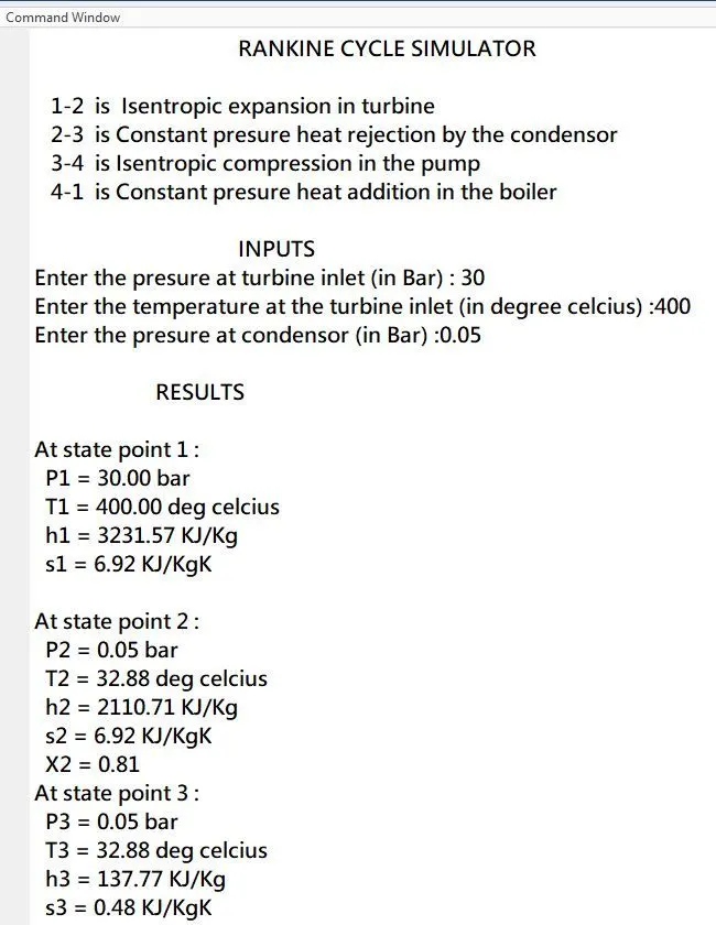
- To find all the state points in the rankine cycle and display in the command window.
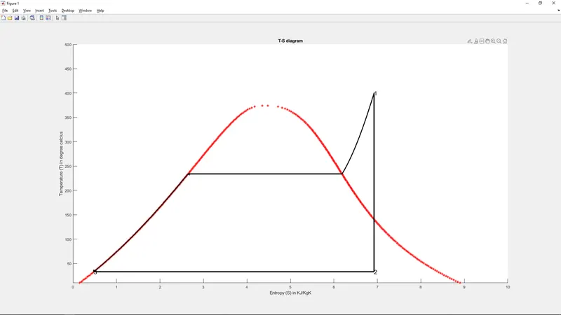
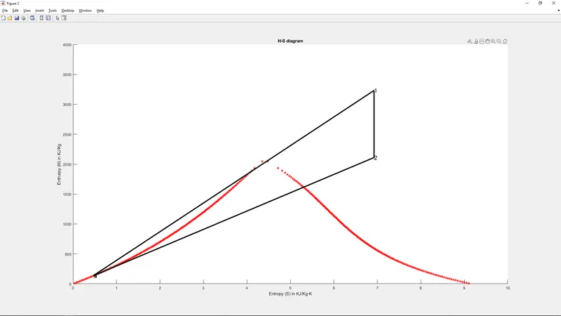
- To plot the T-S ans H-S diagram of rankine cycle for a given input values.
- To calculate the net work output and back work ratio.
Rankine Cycle
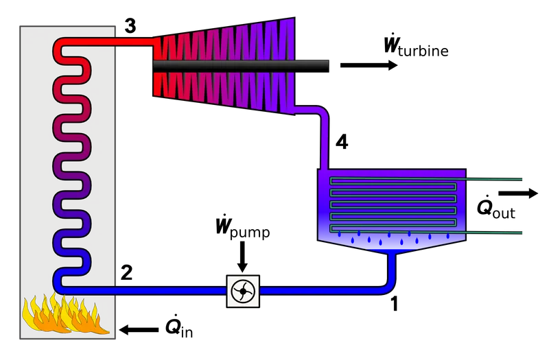
The Rankine cycle is a model used to predict the performance of steam turbine systems. It was also used to study the performance of reciprocating steam engines. The Rankine cycle is an idealized thermodynamic cycle of a heat engine that converts heat into mechanical work while undergoing phase change. It is an idealized cycle in which friction losses in each of the four components are neglected. The heat is supplied externally to a closed loop, which usually uses water as the working fluid.
Process in Rankine cycle
process 1-2 is Isentropic expansion in turbine.
process 2-3 is Constant presure heat rejection by the condensor .
process 3-4 is Isentropic compression in the pump.
process 4-1 is Constant presure heat addition in the boiler.
Formulas Used
Turbine work(Wt) = `h1-h2`
Pump work(Wp) = `h4-h3`
Net work output(Wnet) = `(h1-h2)-(h4-h3)`
Thermal efficiency(Ntherm) = `(1-(h2-h3)/(h1-h4))*100`
Specific Steam Consumption(S.S.C) = `(3600)/((h1-h2)-(h4-h3))`
Back Work ratio = `(h4-h3)/(h1-h2)`
Main code
% Creation of Rankine cycle simulator
clear all
close all
clc

% Process in Rankine cycle
disp('                                     RANKINE CYCLE SIMULATOR                          ')
disp(' ')
disp('   1-2  is  Isentropic expansion in turbine')
disp('   2-3  is Constant presure heat rejection by the condensor ')
disp('   3-4  is Isentropic compression in the pump')
disp('   4-1  is Constant presure heat addition in the boiler')
disp(' ')

% Inputs
disp('                                     INPUTS                   ')
P1 = input('Enter the presure at turbine inlet (in Bar) : ');
T1 = input('Enter the temperature at the turbine inlet (in degree celcius) :');
P2 = input('Enter the presure at condensor (in Bar) :');
disp(' ')

% At State point 1
h1 = XSteam('h_pT', P1,T1);
s1 = XSteam('s_pT', P1,T1);
sf1 = XSteam('sL_p',P1);
sg1 = XSteam('sV_p',P1);
T_sat1 = XSteam('Tsat_p',P1);

% At State point 2
s2 = s1;
sf2 = XSteam('sL_p', P2);
sg2 = XSteam('sV_p',P2);
sfg2 = sg2-sf2;
% Dryness factor
x2 = (s2-sf2)/(sfg2);

hf2 = XSteam('hL_p', P2);
hg2 = XSteam('hV_p', P2);
h2 = hf2 + (x2*(hg2-hf2));
T_sat2 = XSteam('Tsat_p', P2);
T2 = T_sat2;

% At State point 3
h3 = hf2;
s3 = sf2;
P3 = P2;
T3 = T2;

% At State point 4
s4 = s3;
P4 = P1;
h4 = XSteam('h_ps',P4,s4);
cp4 = XSteam('Cp_ps', P4,s4);
cv4 = XSteam('Cv_ps', P4,s4);
k = cp4/cv4;
T4 = T3/(P3/P4)^((k-1)/k);

% Calculation of net work done
turbine_work = h1-h2;
pump_work = h4-h3;
net_work = turbine_work - pump_work;

% Calculation of thermal efficiency
Thermal_efficiency = (1 - (h2-h3)/(h1-h4))*100;
% Back work ratio
back_work = pump_work/turbine_work;
% Specific Steam Consumption
ssc = 3600/net_work;

% Plotting T-S diagram
x = linspace(0,400,200);
figure(1)
hold on
% The saturation curve for Temperature and entropy
for i = 1:length(x)
    plot(XSteam('sL_T' ,x(i)),x(i),'r*')
    plot(XSteam('sV_T' ,x(i)),x(i),'r*')
end
% The curve of temperature and entropy
plot([s1,s2],[T1,T2],'linewidth',3,'color','black')
axis([0,10,10,500])
text(s1,T1,'1','FontSize',15)
if x2 > 1
    T3 = T_sat2;
    T2 = T_sat2;
    plot([s2,sg2,s3,s4],[T2,T_sat2,T3,T4],'linewidth',3,'color','black')

    text(s2,T2,'2','FontSize',15)
    text(s3,T3,'3','FontSize',15)
else
    plot([s2,s3,s4],[T2,T3,T4],'linewidth',3,'color','black')
    text(s2,T2,'2','FontSize',15)
    text(s3,T3,'3','FontSize',15)
end
y = linspace(T1,T2,400);
for j = 1:length(y)
    plot(XSteam('s_pT',P1,y(j)),y(j),'.','linewidth',3,'color','black')
end
plot([sf1,sg1],[T_sat1,T_sat1],'linewidth',3,'color','black')
text(sf1,T_sat1,'4')
title('T-S diagram')
xlabel('Entropy (S) in KJ/KgK')
ylabel('Temperature (T) in degree celcius')

% The saturation curve of Enthalpy and Entropy
figure(2)
hold on
axis([0,10,0,4000])
for i = 1:length(x)
    plot(XSteam('sL_T' ,x(i)),XSteam('hL_T' ,x(i)),'r*')
    plot(XSteam('sV_T' ,x(i)),XSteam('hL_T' ,x(i)),'r*')
end
% The curve of entropy and enthalpy
plot([s1,s2,s3,s4,s1],[h1,h2,h3,h4,h1],'linewidth',3,'color','black')
text(s1,h1,'1','FontSize',15)
text(s2,h2,'2','FontSize',15)
text(s3,h3,'3','FontSize',15)
text(s4,h4,'4','FontSize',15)
title('H-S diagram')
xlabel('Entropy (S) in KJ/Kg-K')
ylabel('Enthalpy (H) in KJ/Kg')

% Results to be shown in command window
disp('                      RESULTS                  ')
% At State point 1
disp(' ')
disp('At state point 1 :')
fprintf('  P1 = %.2f bar \n',P1)
fprintf('  T1 = %.2f deg celcius \n',T1)
fprintf('  h1 = %.2f KJ/Kg \n',h1)
fprintf('  s1 = %.2f KJ/KgK \n',s1)
disp(' ')
% At State point 2
disp('At state point 2 :')
fprintf('  P2 = %.2f bar \n',P2)
fprintf('  T2 = %.2f deg celcius \n',T2)
fprintf('  h2 = %.2f KJ/Kg \n',h2)
fprintf('  s2 = %.2f KJ/KgK \n',s2)
fprintf('  X2 = %.2f',x2)
disp(' ')
% At State point 3
disp('At state point 3 :')
fprintf('  P3 = %.2f bar \n',P3)
fprintf('  T3 = %.2f deg celcius \n',T3)
fprintf('  h3 = %.2f KJ/Kg \n',h3)
fprintf('  s3 = %.2f KJ/KgK \n',s3)
disp(' ')
% At State point 4
disp('At state point 4 :')
fprintf('  P4 = %.2f bar \n',P4)
fprintf('  T4 = %.2f deg celcius \n',T4)
fprintf('  h4 = %.2f KJ/Kg \n',h4)
fprintf('  s4 = %.2f KJ/KgK \n',s4)
disp(' ')
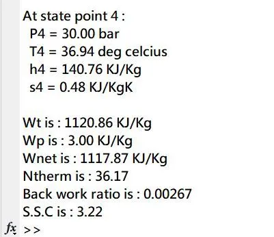
fprintf('Wt is : %.2f KJ/Kg \n',turbine_work)
fprintf('Wp is : %.2f KJ/Kg \n', pump_work)
fprintf('Wnet is : %.2f KJ/Kg \n', net_work)
fprintf('Ntherm is : %.2f \n',Thermal_efficiency)
fprintf('Back work ratio is : %.5f \n', back_work)
fprintf('S.S.C is : %.2f \n', ssc)
Explanation
This operation is done by the program language MATLAB.
Open Matlab software and start to type the command.
Write clear all, close all and clc command to clear previous command and close previous figure windows.
Display the process in rankine cycle on the command window by using disp command.
Get the initial inputs for temperature and presure from the user by using input command.
Find the entropy, enthalpy, Temperature and presure at different state point from 1 to 4
Get the values of saturated liquid and vapour values of entalpy entropy and temperature by using XSteam function for every state point.
Hence we obtain the values of enthalpy, entropy, Temperature and presure at all state point.
With the help of above formula Net work output, Thermal efficiency and specific steam consumption can be calculated.
As ploting the graph for T-S diagram, first find the saturation curve by using different set of values in temperature and entropy in the XSteam function. Loop the program to get multiple values.
Plot the first state point values of temperature and entropy in the graph.
For the second and third state point there are two possibilities.
- If the Dryness factor(x2) is greater than 1 then the value os T3 = T_sat2
- If it is not grater than 1 then there will be no change in values of temperature in ploting graph.
Plot the fourth state point of temperature and entropy in the graph
For finding the H-S diagram, find the saturation curve by using different set of values in temperature and entropy in the XSteam function. Loop the program to get multiple values.
Plot the obtained values of enthalpy and entropy in the different state points in the graph.
With the help of fprintf command display the values of Presure, Temperature, enthalpy and entropy at different state points in the command window.
Also display the Net work output, back work ration, Thermal efficiency and specific steam consumption in the command window.
T-S diagram of Rankine cycle
H-S diagram of rankine cycle
The results in command window
Errors faced
1. I forgot to add h1 and s1 to the plot for graph to complete.
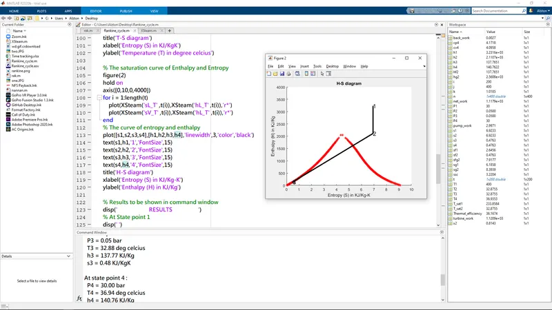
I corrected by adding those variables.
2. I misplaced the variable T1 instead of P1
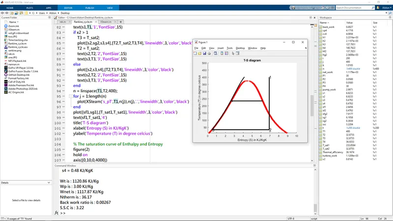
I rectified it by placing correct variable in it.
Conclusion
The rankine cycle simulator is created sucessfully by using matlab program
The state points in the rankine cycle is calculated and it was shown in the command window
The graphs of T-S and H-S diagram for the rankine cycle is plotted sucessfully.
The values of net work output and back work ratio are also calculated.
References