Project 2 - Rankine cycle Simulator

Aim:

Understand the concept of Rankine cycle by referring to standard thermal engineering text book.

Objectivies:

By creating a Rankine simulator using Matlab, calculate the state points of the Rankine cycle based on given inputs. Addition to that plot the corresponding T-s and h-s plots.

Theory of Rankine cycle:

Rankine cycle or Rankine vapor cycle is the process widely used by power plants such as coal-fired power plants or neculear reactors. In this mechanism, the fuel is used to produce heat within a boiler, converting water into steam which then expands through a turbine producing useful work. This process was developed in 1859 by Sottish engineer William J.M. Rankine. This is a thermodynamic cycle which converts heat into mechanical energy-which usually gets transformed into electricity by electricity generation.

A simple illustration with components for the Rankine Cycle:

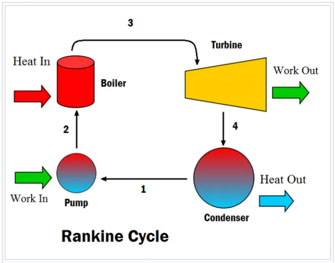
Figure-1

The presssure volume diagram for the Rankine Cycle. This illustrates the changes in pressure and volume the working fluid(water) undergoes to produce work.

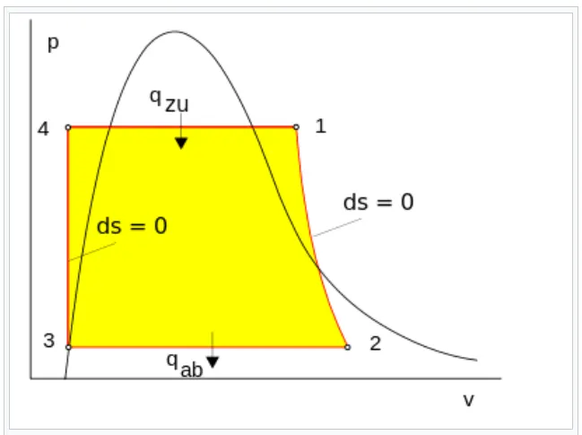
Figure-2

Pump: Compression of the fluid to high pressure using a pump (this takes work) (Figure-2: Steps 3 to 4)

w_{pump, in} = h4 - h3

Boiler: The compressed fluid is heated to the final temperature(which is at boiling point), therefore, a phase change occurs - from liquid to vapor (Figure-2: Steps 4 to 1)

q_in = h1 - h4

Turbine: Expansion of the vapor in the turbine. (Figure-2: Steps 1 to 2)

w_{turbine, out} = h2 - h1

Condenser: Condensation of the vapor in the condenser, where the waste heat goes to final heat sink (the atmosphere or a large body of water, ex - lake or river) (Figure-2: Steps 2 to 3)

q_out = h2 - h3

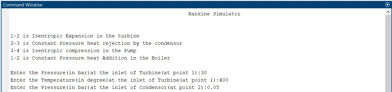
1-2 is Isentropic Expansion in the turbine

2-3 is Constant Pressure heat rejection by the condensor

3-4 is Isentropic compression in the Pump

1-2 is Constant Pressure heat Addition in the Boiler

The efficiency of the Rankine cycle is limited by the high heat of vaporization by the fluid. The fluid must be cycled through and reused constantly, therefore, water is the most practical fluid for this cycle. This is not why many power plants are located near a body of water – that is for the waste heat.

As the water condenses in the condenser, waste heat is given off in the form of waste vapor—which can be seen billowing from a plant's cooling towers. This waste heat is necessary in any thermodynamic cycle. Due to this condensation step, the pressure at the turbine outlet is lowered. This means the pump requires less work to compress the water—resulting in higher overall efficiencies.

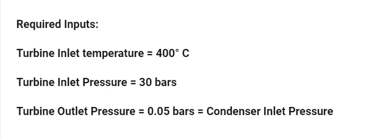
Based on above said understanding of Rankine theory and process steps, Programming code has been written as below:

CODES:

clear all
close all
clc

% User inputs
fprintf('%75s','Rankine Simulator');
fprintf('\n\n\n')
fprintf('1-2 is Isentropic Expansion in the turbine \n');
fprintf('2-3 is Constant Pressure heat rejection by the condensor \n');
fprintf('3-4 is Isentropic compression in the Pump \n');
fprintf('1-2 is Constant Pressure heat Addition in the Boiler \n\n');

%inputs
p1 = input('Enter the Pressure(in bar)at the inlet of Turbine(at point 1):');
t1 = input('Enter the Temperature(in degree)at the inlet of Turbine(at point 1):');
p2 = input('Enter the Pressure(in bar)at the inlet of Condensor(at point 2):');

%inputs to the Turbine
s1 = XSteam('s_pT',p1,t1);
h1 = XSteam('h_pT',p1,t1);

%Condensor inlet
s2 = s1; % 1-2 is Isentropic expansion process
sf2 = XSteam('sL_p' ,p2);
sg2 = XSteam('sV_p' ,p2);
hf2 = XSteam('hL_p' ,p2);
hg2 = XSteam('hV_p' ,p2);

% Calculating Dryness fraction
if(s2<=sg2)
   x2 = ((s2 - sg2)/ (sf2 - sg2)); % Dryness fraction at state point 2 
else
    x2 = 1;
end
h2 = hf2+(hg2 - hf2);

% Condensor exit
p3 = p2;
t3 = XSteam('Tsat_p',p3);
s3 = XSteam('sL_p',p3);
h3 = XSteam('hL_p',p3);
v3 = XSteam('vL_p',p3);
t2 = t3;

% Boiller inlet
p4 = p1; % Constant Heat Addition
s4 = s3; % Isentrpic compression in the pump
h4 = XSteam('h_ps', p4, s4);
cp4 = XSteam('cp_ps', p4, s4);
cv4 = XSteam('cv_ps', p4, s4);
g4 = (cp4/cv4);
% Calculation for t4
%p4^(1-gamma)*t4^gamma = p3^(1-gamma)*t3^gamma
t4 = (t3*((p3/p4)^((1-g4)/g4)));

% Calculations
% work done by the turbine
Wt = h1 - h2;

% work done by the pump
Wp = h4 - h3;

% net work done
W_net = Wt - Wp;

% Heat added in the boiler
q_in = h1 - h4;

% Heat rejecteded in the condensor
q_out = h2 - h3;

% Thermal efficiency
n = (W_net/q_in)*100;

% Plotting the results

figure(1)

% Plotting liquid and vapour curves
t = linspace(1,t1,1000);
for i = 1:length(t)
    s_l(i) = XSteam('sL_T',t(i));
end

for i = 1:length(t)
    s_v(i) = XSteam('sV_T',t(i));
end
hold on
plot(s_l,t,'linewidth',2,'linestyle','- -','color','r');
plot(s_v,t,'linewidth',2,'linestyle','- -','color','r');
grid on

% Plotting for the work done by the turbine (Process 1 - 2)
plot([s1,s2],[t1,t2],'linewidth',2,'color','b');
hold on
title('T-s Diagram of Ideal Rankine Cycle');
xlabel('Entropy(KJ/KgK)');
ylabel('Temperature(k)');

% Plotting for heat rejection in Condensor (Process 2 - 3)
plot([s2,s3],[t2,t3],'linewidth',2,'color','b');
hold on


% Plotting for the work done by the Pump (Process 3 - 4)
plot([s3,s4],[t3,t4],'linewidth',2,'color','b');
hold on

% Plotting for heat addition by the Boiler (Process 4 - 1)
tp = XSteam ('TSat_p', p4);
sp = XSteam ('sL_T',tp);
plot([s4,sp],[t4,tp],'linewidth',2,'color','b');
hold on

tq = tp;
sq = XSteam ('sV_T',tq);
plot([sp,sq],[tp,tq],'linewidth',2,'color','b');
hold on

plot([sq,s1],[tq,t1],'linewidth',2,'color','b');
hold on

% Indicate states with numbers
text (s1,t1, '1')
text (s2,t2, '2')
text (s3,t3, '3')
text (s4,t4, '4')

% Plot for Enthalpy vs Entropy
figure(2)

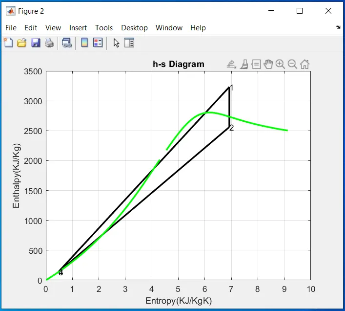
plot([s1,s2], [h1,h2],'linewidth',2,'color','black');
grid on
title('h-s Diagram')
xlabel('Entropy(KJ/KgK)')
ylabel('Enthalpy(KJ/Kg)')
hold on

plot([s2,s3], [h2,h3],'linewidth',2,'color','black');
hold on

plot([s3,s4], [h3,h4],'linewidth',2,'color','black');
hold on

plot([s4,s1], [h4,h1],'linewidth',2,'color','black');
hold on

% Plotting liquid and vapour saturation curves
t = linspace(1,t1,1000);
for j = 1:length(t)
    h_l(j) = XSteam('hL_T',t(j));
end

for j = 1:length(t)
    h_v(j) = XSteam('hV_T',t(j));
end

plot(s_l,h_l,'linewidth',2,'color','g');
hold on
plot(s_v,h_v,'linewidth',2,'color','g');


% Indicate states with numbers
text (s1,h1, '1')
text (s2,h2, '2')
text (s3,h3, '3')
text (s4,h4, '4')
 

% Results output
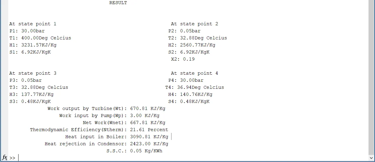
fprintf('%40s \n\n\n','RESULT');
fprintf('%10s %54s \n','At state point 1','At state point 2');
fprintf('%s %.2f%s %44s %.2f%s \n','P1:',p1,'bar','P2:',p2,'bar');
fprintf('%s %.2f%s %35s %.2f%s \n','T1:',t1,'Deg Celcius','T2:',t2,'Deg Celcius');
fprintf('%s %.2f%s %40s %.2f%s \n','H1:',h1,'KJ/Kg','H2:',h2,'KJ/Kg');    
fprintf('%s %.2f%s %42s %.2f%s \n','S1:',s1,'KJ/KgK','S2:',s2,'KJ/KgK');     
fprintf('%58s %.2f \n\n','X2:',x2);    
fprintf('%10s %54s \n','At state point 3','At state point 4');
fprintf('%s %.2f%s %45s %.2f%s \n','P3:',p3,'bar','P4:',p4,'bar');
fprintf('%s %.2f%s %35s %.2f%s \n','T3:',t3,'Deg Celcius','T4:',t4,'Deg Celcius');
fprintf('%s %.2f%s %41s %.2f%s \n','H3:',h3,'KJ/Kg','H4:',h4,'KJ/Kg');
fprintf('%s %.2f%s %42s %.2f%s \n','S3:',s3,'KJ/KgK','S4:',s4,'KJ/KgK');


fprintf('%40s %.2f %s \n','Work output by Turbine(Wt):',Wt,'KJ/Kg');
fprintf('%40s %.2f %s \n','Work input by Pump(Wp):',Wp,'KJ/Kg');
fprintf('%40s %.2f %s \n','Net Work(Wnet):',W_net,'KJ/Kg');
fprintf('%40s %.2f %s \n','Thermodynamic Efficiency(Ntherm):',n,'Percent');
fprintf('%40s %.2f %s \n','Heat input in Boiler:',q_in,'KJ/Kg');
fprintf('%40s %.2f %s \n','Heat rejection in Condensor:',q_out,'KJ/Kg');
fprintf('%40s %.2f %s \n','S.S.C.:',p3,'Kg/KWh');

Results:

T -s diagram:

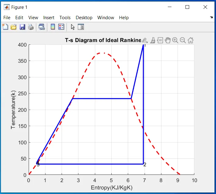
h-s diagram:

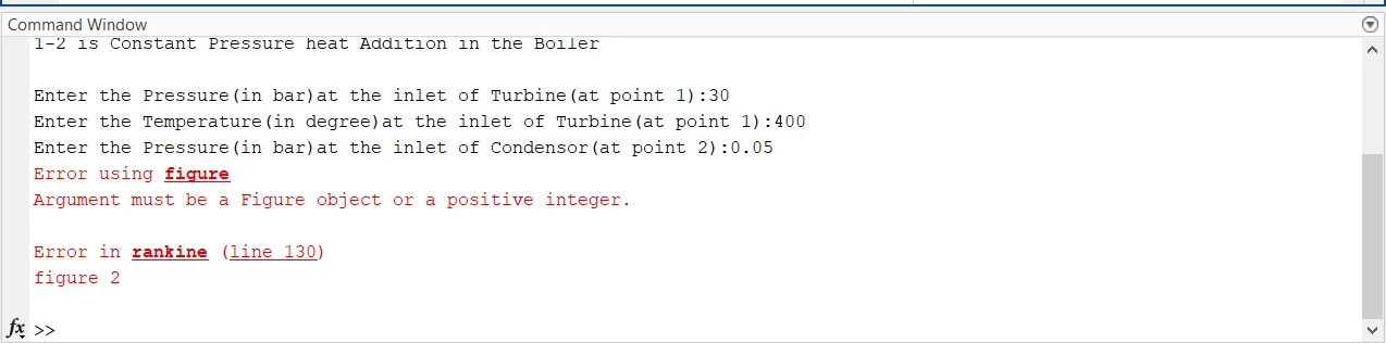
Error faced:

Error fixed:

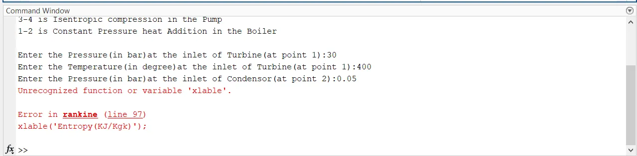
Errors occured due to typo error, after writing codes, read through the whole program line by line carefully and fixed any missing arguments, typo error so on.

Explanation of codes:

Function XSteam - which is the steam table

Dryness fraction - which is helpful to calculate the actual Enthalpy of wet steam

For understanding and knowledge: Reference only

The steam dryness fraction is used to quantify the amount of water within steam.

• Dry steam - all water molecules are in the gaseous state
• Wet steam - a portion of the water molecules have lost their energy - latent heat - and condensed to tiny water droplets

To produce 100% dry steam in an boiler and keep the steam dry throughout the piping system is in general not possible. Droplets of water will escape from the boiler surface due to turbulence and splashing when bubbles of steam break through the water surface. The steam leaving the boiler space will contain a mixture of water droplets and steam.

In addition heat loss in the pipe lines condensates parts of the steam to droplets of water.

Steam - produced in a boiler where the heat is supplied to the water and where the steam is in contact with the water surface of the boiler - contains approximately 5% water by mass.

Dryness fraction of Wet Steam

If the water content in the steam is 5% by mass, then the steam is said to be 95% dry with a dryness fraction 0.95.

Dryness fraction can be expressed:

ζ = w_s / (w_w + w_s) (1)

where

ζ = dryness fraction

w_w = mass of water (kg, lb)

w_s = mass of steam (kg, lb)

Enthalpy of Wet Steam

Actual enthalpy of wet steam can be calculated with the dryness fraction - ζ - and the specific enthalpy - h_s - of "dry" steam picked from steam tables. Wet steam will always have lower usable heat energy than "dry" steam.

h_t = h_s ζ + (1 - ζ ) h_w (2)

where

h_t = enthalpy of wet steam (kJ/kg, Btu/lb)

h_s = enthalpy of "dry" steam (kJ/kg, Btu/lb)

h_w = enthalpy of saturated water or condensate (kJ/kg, Btu/lb)

Specific Volume of Wet Steam

The droplets of water in wet steam occupies a negligible space in the steam and the specific volume of wet steam will be reduced by the dryness fraction.

v_t = v_s ζ (3)

where

v_t = specific volume of wet steam (m³/kg, ft³/lb)

v_s = specific volume of the dry steam (m³/kg, ft³/lb)

Example - Enthalpy and Specific Volume of Wet Steam

Steam with pressure 5 bar gauge (6 bar abs) has a dryness fraction of 0.95. From the steam table

h_s = 2755.46 (kJ/kg)

h_w = 670.43 (kJ/kg)

The total enthalpy can be calculated:

h_t = (2755.46 kJ/kg) 0.95 + (1 - 0.95) (670.43 kJ/kg)

= 2651 kJ/kg

Specific volume can be calculated:

v = (0.315 m³/kg) 0.95

= 0.299 m³/kg

Results:

Thus with the help of standard XSteam library to get the steam table date for water, the Rankine Cycle simulator has been created using Matlab. In addition, the net work output, back work ratio were calculated. T-s diagram and h-s diagram were plotted.

Understood how the Rankine cycle efficiency can be improved.

References:

https://en.wikipedia.org/wiki/Rankine_cycle

https://www.nuclear-power.net/nuclear-engineering/thermodynamics/thermodynamic-cycles/rankine-cycle-steam-turbine-cycle/theory-of-rankine-cycle-equations-and-calculation/

https://energyeducation.ca/encyclopedia/Rankine_cycle

https://www.engineeringtoolbox.com/wet-steam-quality-d_426.html

https://www.electrical4u.com/rankine-cycle-efficiency-improvement-techniques/