Performing a Curve fitting using Matlab
Aim:
To accomplish a Curve fitting for a given dataset and to realise the best and perfect fit for that particular dataset using Matlab.
Understanding of Curve fitting:
Curve fitting is the process of constructing a curve or mathematical function, that has the best fit to a series of data points, possibly subject to constraints. Curve fitting can involve either interpolation, where an exact fit to the data is required, or smoothing, in which a “smooth” function is constructed that approximately fits the data. Interpolation is used to estimate the data points between to known points. The most common interpolation technique is Linear interpolation, but there are types available such as:
- nearest
- spline
- cubic
- etc.,
Uses of Curve fitting:
Curve fit is immensely powerful, and it is helpful that how our data changes mathematically and once have a curve fit, we can actually do the additional mathematics operation which might not be possible in the initial dataset.
Objectives:
The main objectives of this project are how to make the curve fit perfectly, how to get the best fit and what could be done to improve the cubic fit for the given dataset.
For this purpose, write a code fit a linear and cubic polynomial for the Cp data and write a code to show splitwise method. With these different methods we are going to analyse and try to come to the conculation as which one is the best and perfect fit for the particular given dataset.
In this project, we take specific Heat data for oxyzen as a function of time.
Parameters used to measure the fitness characteristics of both curves which are original curve and fitted curve:
Below listed four quantities which helps us the goodness of fit requirements or how well the equation is representing the data points upon finding a curve which satisfies the data points:
The sum of squares due to error (SSE)
`SSE = sum_(i=1)^n (Y(i)-f(x(i)))^2`
The sum of squares of squares of regression (SSR)
`SSR = sum_(i=1)^n (f(x(i))-Mean)^2`
Now the term SST is given by the summation of SSR and SSE
`SST = SSE +SSR`
From here, we can calculate the value of R^2,
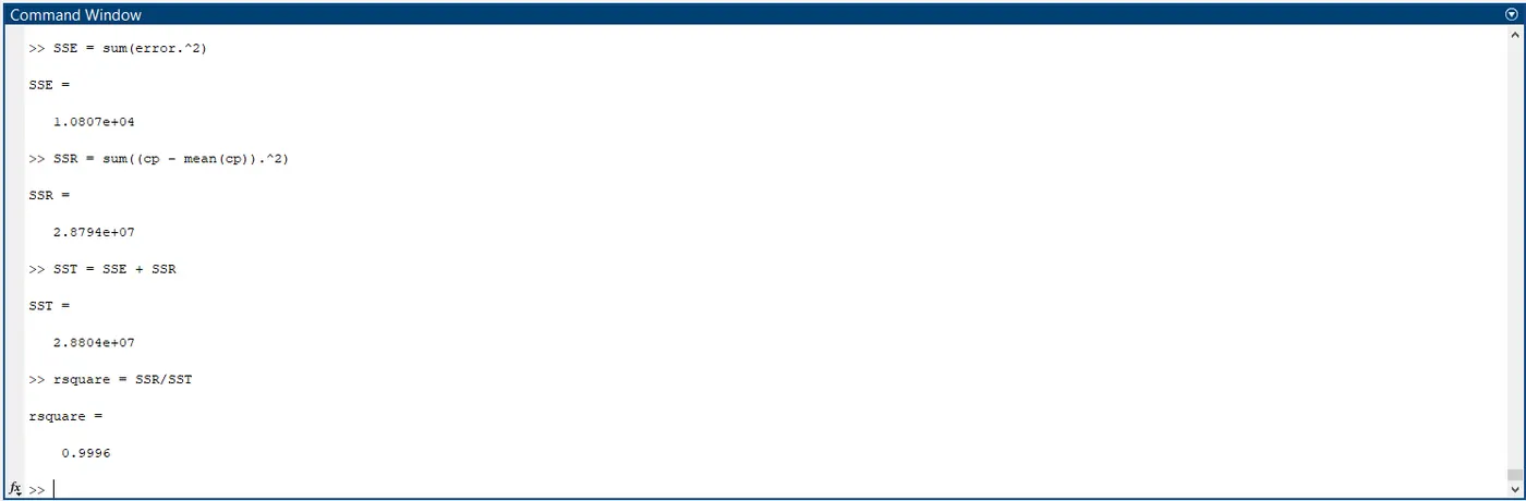
`R^2=(SSR)/(SST)`
`RMSE = sqrt(SSE)/n`, where n = Total number of data points available
Initial codes to construct the Curve fit with given dataset:
Linear fit:
clear all
close all
clc

% Preparing the data

cp_data = load('data');
temperature = cp_data(:,1);
cp = cp_data(:,2);
mean_cp = mean(cp);
n = 3200;

%Curve fit

% cp = a*T+b

co_effs = polyfit(temperature,cp,1);
predicted_cp = polyval(co_effs, temperature);

% Compare my curve fit with original data

figure(1)
plot(temperature, cp, 'linewidth', 3)
hold on
plot(temperature, predicted_cp, 'linewidth',3, 'color', 'r');
xlabel('Temperature [K]');
ylabel('Specific Heat [KJ/Kmol-K]');
title('Linear Polynomial curve fit');
legend('Original dataset', 'Curve fit');
grid on

% Calculation of Goodness fit of linear polynomial
error = cp - predicted_cp;
sse_linear = sum(error.^2);
ssr_linear = sum((cp - mean(cp)).^2);
sst_linear = sse_linear + ssr_linear;
rsquare_linear = ssr_linear/sst_linear;
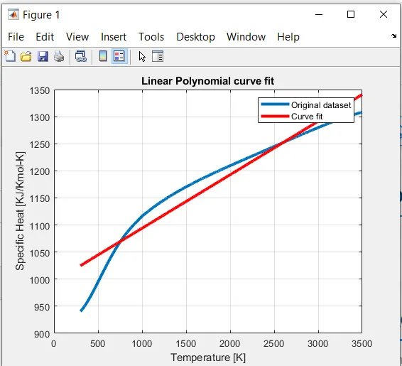
Output plot for the above code - Linear fit:
R^2 Out put which is clearly interpret the best fit:

Explanation of codes:
clear all - is used to clear all the previous variables
close all - is used to clear all the previously plotted graphs
clc - is used to clear the command window
% Preparing the data
cp_data = load('data'); - is used to load the given data from the sourcing folder.
temperature = cp_data(:,1); - is the temperature data given in the first coloumn of dataset.
cp = cp_data(:,2); - is the specific Heat data given in the second coloumn of dataset.
To obtain comparison curve fitting_linear:
%Curve fit
% cp = a*T+ b
co_effs = polyfit(temperature,cp,1);
predicted_cp = polyval(co_effs, temperature);
Codes for plotting:
% Compare my curve fit with original data
figure(1)
plot(temperature, cp, 'linewidth', 3)
hold on
plot(temperature, predicted_cp, 'linewidth',3, 'color', 'r');
xlabel('Temperature [K]');
ylabel('Specific Heat [KJ/Kmol-K]');
title('Linear Polynomial curve fit');
legend('Original dataset', 'Curve fit');
grid on
Codes for calculations:
% Calculation of Goodness fit of linear polynomial
error = cp - predicted_cp; - is used to calculate the error
sse_linear = sum(error.^2); - is used to calculate the sum of squared error
ssr_linear = sum((cp - mean(cp)).^2); - is used to calculate the sum of squares of regression
sst_linear = sse_linear + ssr_linear; - is used to calculate the sum of total of sum square error and sum square regression
rsquare_linear = ssr_linear/sst_linear; - is used to calculate the value of R^2
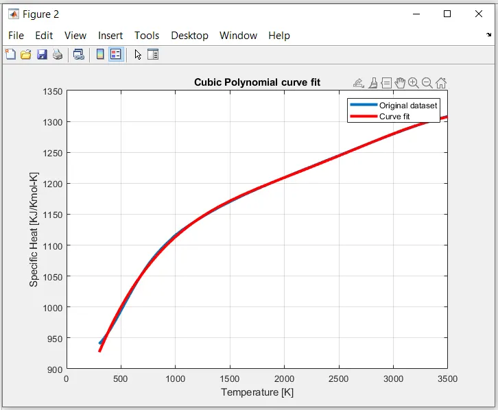
With this method of linear curve fitting, we understood that the curve fitting is not seems to be good, so that, write a code for cubic curve fitting to plot the curve fit and calculate the `R^2` value, where `R^2` is >.95 to perform a perfect fit.
Codes for cubic curve fitting method with 5th degree polynomial:
clear all
close all
clc

% Preparing the data

cp_data = load('data');
temperature = cp_data(:,1);
cp = cp_data(:,2);
mean_cp = mean(cp);
n = 3200;

%Curve fit_Cubic curve fitting

% cp_cubic = a*T^2+b*T+C

co_effs = polyfit(temperature,cp,5);
predicted_cp = polyval(co_effs, temperature);

% Compare my curve fit with original data

figure(2)
plot(temperature, cp, 'linewidth', 3)
hold on
plot(temperature, predicted_cp, 'linewidth',3, 'color', 'r');
xlabel('Temperature [K]');
ylabel('Specific Heat [KJ/Kmol-K]');
title('Cubic Polynomial curve fit');
legend('Original dataset', 'Curve fit');
grid on

% Calculation of Goodness fit of Cubic polynomial
error = cp - predicted_cp;
sse_cubic = sum(error.^2);
ssr_cubic = sum((cp - mean(cp)).^2);
sst_cubic = sse_cubic + ssr_cubic;
rsquare_cubic = ssr_cubic/sst_cubic;
Plotting Cubic Curve fitting:
R^2 Out put which perform the best fit in Cubic method:
Improvement of Cubic Polynomial curve fitting with Splitwise method:
clear all
close all
clc

% Preparing the data

cp_data = load('data');
temperature = cp_data(:,1);
cp = cp_data(:,2);
mean_cp = mean(cp);
n = 3200;

%Cubic curve fitting_Splitwise method

% cp_cubic = a*T^2+b*T+C

temperature_1 = cp_data(1:400,1);
cp_1 = cp_data(1:400,2);
co_effs_1 = polyfit(temperature_1,cp_1,4);
predicted_cp_1 = polyval(co_effs_1, temperature_1);

temperature_2 = cp_data(401:800,1);
cp_2 = cp_data(401:800,2);
co_effs_2 = polyfit(temperature_2,cp_2,4);
predicted_cp_2 = polyval(co_effs_2, temperature_2);

temperature_3 = cp_data(801:1200,1);
cp_3 = cp_data(801:1200,2);
co_effs_3 = polyfit(temperature_3,cp_3,4);
predicted_cp_3 = polyval(co_effs_3, temperature_3);

temperature_4 = cp_data(1201:1600,1);
cp_4 = cp_data(1201:1600,2);
co_effs_4 = polyfit(temperature_4,cp_4,4);
predicted_cp_4 = polyval(co_effs_4, temperature_4);

temperature_5 = cp_data(1601:2000,1);
cp_5 = cp_data(1601:2000,2);
co_effs_5 = polyfit(temperature_5,cp_5,4);
predicted_cp_5 = polyval(co_effs_5, temperature_5);

temperature_6 = cp_data(2001:2400,1);
cp_6 = cp_data(2001:2400,2);
co_effs_6 = polyfit(temperature_6,cp_6,4);
predicted_cp_6 = polyval(co_effs_6, temperature_6);

temperature_7 = cp_data(2401:2800,1);
cp_7 = cp_data(2401:2800,2);
co_effs_7 = polyfit(temperature_7,cp_7,4);
predicted_cp_7 = polyval(co_effs_7, temperature_7);

temperature_8 = cp_data(2801:3200,1);
cp_8 = cp_data(2801:3200,2);
co_effs_8 = polyfit(temperature_8,cp_8,4);
predicted_cp_8 = polyval(co_effs_8, temperature_8);

% Plotting Original dataset
plot(temperature, cp, 'linewidth',3,'color','r');
hold on

% Splitwise Dataset
predicted_cp = [predicted_cp_1; predicted_cp_2; predicted_cp_3; predicted_cp_4; predicted_cp_5; predicted_cp_6; predicted_cp_7; predicted_cp_8]
plot(temperature, predicted_cp, 'linewidth',1.5,'color','k');

xlabel('Temperature (K)');
ylabel('Specific Heat (KJ/Kmol-K)');
title('Splitwise Method');
legend('Original Dataset','Splitwise Dataset')
grid on


% For loop to calculate repeated values with 8 different set of temperature dataset

for i = 1:length(cp);
    error_splitwise = cp(i) - predicted_cp(i);
    sse_cubic_splitwise = sum(error_splitwise).^2;
    ssr_cubic_splitwise = sum((predicted_cp(i) - mean(cp)).^2);
end

% Calculation of Goodness fit of Cubic polynomial with Splitwise Method

sst_cubic_splitwise = sse_cubic_splitwise + ssr_cubic_splitwise;
rsquare_cubic_splitwise = ssr_cubic_splitwise/sst_cubic_splitwise;
rmse_cubic_splitwise = sqrt(sse_cubic_splitwise/n);
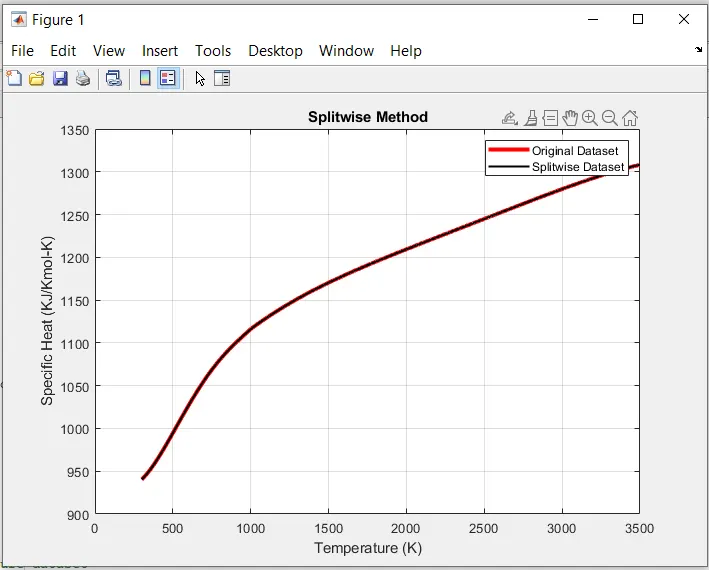
Plotting for Splitwise Method:
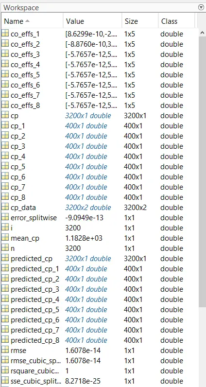
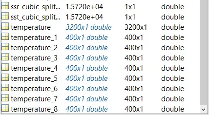
Splitwise workspace:
Explanation of Splitwise codes:
To improve and obtain the goodness of curve fit , we split the given temperature data into 8 groups to get 8 difference of splitting cp, and executes this program . From there we can achieve perfect curve fit with individual segment of plotting and nesting these segemnts into one exact curve.
temperature_1 = cp_data(1:400,1);
cp_1 = cp_data(1:400,2);
co_effs_1 = polyfit(temperature_1,cp_1,4);
predicted_cp_1 = polyval(co_effs_1, temperature_1);
temperature_2 = cp_data(401:800,1);
cp_2 = cp_data(401:800,2);
co_effs_2 = polyfit(temperature_2,cp_2,4);
predicted_cp_2 = polyval(co_effs_2, temperature_2);
temperature_3 = cp_data(801:1200,1);
cp_3 = cp_data(801:1200,2);
co_effs_3 = polyfit(temperature_3,cp_3,4);
predicted_cp_3 = polyval(co_effs_3, temperature_3);
temperature_4 = cp_data(1201:1600,1);
cp_4 = cp_data(1201:1600,2);
co_effs_4 = polyfit(temperature_4,cp_4,4);
predicted_cp_4 = polyval(co_effs_4, temperature_4);
temperature_5 = cp_data(1601:2000,1);
cp_5 = cp_data(1601:2000,2);
co_effs_5 = polyfit(temperature_5,cp_5,4);
predicted_cp_5 = polyval(co_effs_5, temperature_5);
temperature_6 = cp_data(2001:2400,1);
cp_6 = cp_data(2001:2400,2);
co_effs_6 = polyfit(temperature_6,cp_6,4);
predicted_cp_6 = polyval(co_effs_6, temperature_6);
temperature_7 = cp_data(2401:2800,1);
cp_7 = cp_data(2401:2800,2);
co_effs_7 = polyfit(temperature_7,cp_7,4);
predicted_cp_7 = polyval(co_effs_7, temperature_7);
temperature_8 = cp_data(2801:3200,1);
cp_8 = cp_data(2801:3200,2);
co_effs_8 = polyfit(temperature_8,cp_8,4);
predicted_cp_8 = polyval(co_effs_8, temperature_8);
Results and Conculation:
Hence, as per given task, we write a different methods of program (Linear and Cubic) to calculate and plot the curve fitting, we came to the conculation of Cubic polynomial method is the perfect curve fitting method and we could understood that by improving the goodness of curve fitting by the program of splitwise method.
References:
1. https://en.wikipedia.org/wiki/Curve_fitting
2. https://skill-lync.com/projects/Curve-Fitting-and-criterion-to-choose-best-fit-41860