Solving second order ODE with the example of Simple pendulum
- AIM:
Write a program in Matlab to solve second order equation. For this we must understand with small example with pendulum.
- Understanding of Pendulum:
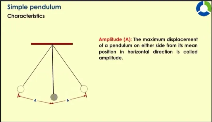
A pendulum is a weight suspended from a pivot so that it can swing freely. When a pendulum is displaced sideways from its resting, equilibrium position, it is restoring force due to gravity that will accelerate it back toward to the equilibrium. When released, the restoring force acting on the pendulum’s mass causes it to oscillate about the equilibrium position, swinging back and forth. The time for on complete cycle, a left and a right swing, is called period. The period depends on the length of the pendulum and to a slight degree on the amplitude, the width of the pendulum’s swing.
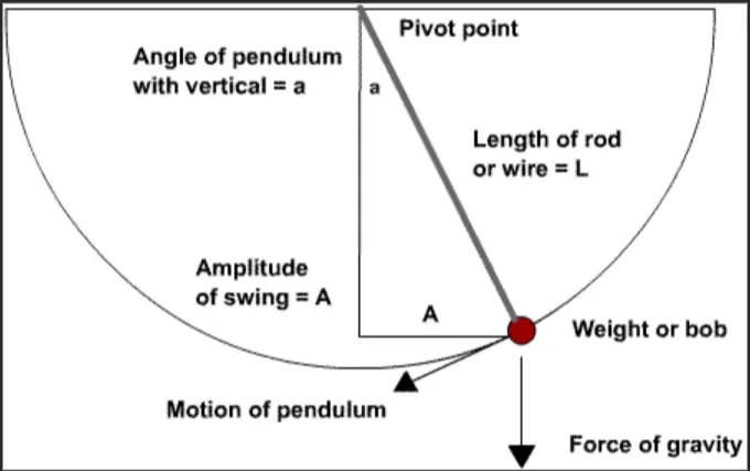
3. Explanation for the Simple pendulm:
Period of pendulum displacement can be calculated by below formula:
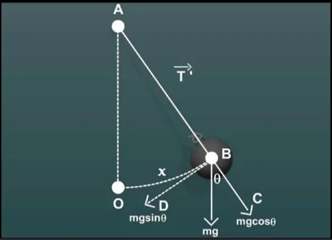
By defining the displacement of the arc length 'x'`from the illustration picture that the net force on the weight is tangent to arc and equals -mxsin`theta`
`F = -mgsintheta`
Tension on the string exactly cancel the component mgcos`theta` parallel to the string. This leaves the net storing force back toward the equilibrium position `theta = 0`
`C = mgcostheta`
The restoring force is directly proportional to the displacement, once the weight releases and oscillate make small angles (less than about 15), `sin theta ~~theta`, Thus the restoring force is
`F~~-mg theta`
The displacement of x is directly proportional `theta`. When `theta` is expressed in radians, the arc length in a circle is related to its radius (L in this example),
`x = Ltheta`
so that,
`theta = s/L`
For small angles, then the expression for the restoring force is:
`F~~-(mg)/Ls`
The expression is of the form:
`F=-ks`
where the force constant is given by `k=(mg)/L`
Using this equation, we can find the period of pendulum for amplitudes with small angles (less than about 15), For a simple pendulum,
`T~~2pisqrt(L/g)`
4. Objectives:
Ordinary Differencial Equation:
In mathematics, an ordinary differencial equation is a differencial equation one or more functions of one independent variable and the derivatives of those functions. The term ordinary is used in contrast with the term partial differencial equation which may be with respect to more than one independent variable.
Second order ODE:
Second order ODE is most important in engineering, it describes a lot of important phenomenon and solving this ODE is understanding the system. A Simple pendulum is the very good example to solve the second order ODE.
The way the pendulum moves depends on the Newton's law.When the law write down, we get a second order Ordinary Differencial Equation that describes the position of the ball with respect to time.
5. Governing Equation:
Standard form of a second order ODE:
`(d^2y)/dx^2+b(dy)/dx+cy=r(x)`
Second order differential equation for a Simple pendulum:
Position and velocity of the weight with respect to time can be determined by solving the second order ODE by using Simple pendulum in Matlab. In order to solve the second ODE, we first break the higher order differenticals to lower order differentials.
`(d^2theta)/dt^2+b/m.(d theta)/dt+g/l.sin theta=0`
where,
b = damping co-efficient,
m = mass of the bob (kg),
l = length of the string (m),
g = acceleration of gravity (m/s^2)
consider,
`theta = theta1`
`d theta/dt=(d theta_1)/dt=theta_2`
then,
`(d^2theta)/dt^2=(d^2theta_1)/dt^2=d/dt(d theta_1/dt)=d(theta^2)`
from this we apply this equation in above simple pendulum ODE:
`(d^2theta)/dt+b/m(d theta_1/dt)+g/l*sin theta_1=0`
`d theta_2/dt+b/m(theta_2)+g/l*sin(theta_1)=0`
`d theta_2/dt=-b/m(theta_2)-g/l*sin(theta_1)`
and now forming the matrix,
`(d theta_1)/dt=theta_2`
`d theta_2/dt=-b/m(theta_2)-g/l*sin(theta_1)`
Matrix,
`d/dt[[theta_1],[theta_2]]=[[theta_2] , [-b/m(theta_2)-g/l*sin(theta_1)]]`
Solving the matrix will leave us with theta1 and theta which can be helped to solve ODE in Simple pendulum.
Program in Matlab for solving ODE:
% Cleaning the screen,Command line,Work space, closing all plots

clear all
close all
clc

% inputs

b=0.05;
l=1; %length of the string in m
g=9.81; %Gravity in m/s^2
m=1; %Mass in kg

% Initial conditions

theta_0=[0;3];

% Time span

t_span=linspace(0,20,500);

% [t,Results]=ode45('ode_func',t_span,theta_0);

[t,Results]=ode45(@(t,theta) ode_func(t,theta,b,g,l,m),t_span,theta_0);
subplot(5,4,[13,14,17,18]);

% Plotting
figure(1)
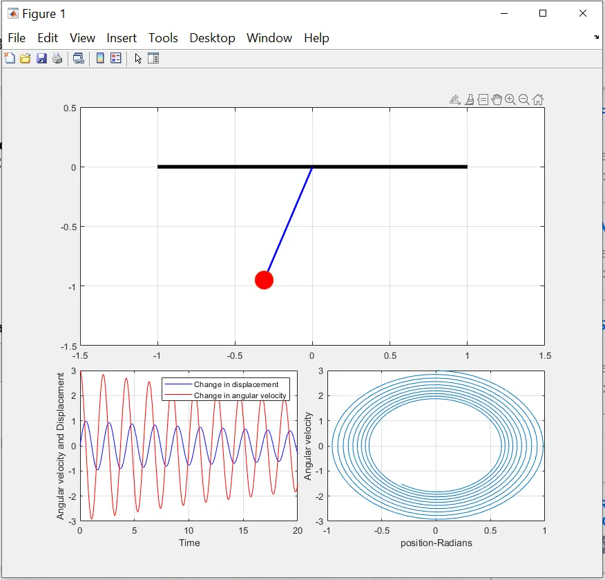
plot(t,Results(:,1),'color','b');
hold on;
plot(t,Results(:,2),'color','r');
grid on;
xlabel('Time');
ylabel('Angular velocity and Displacement');
legend('Change in displacement','Change in angular velocity');
hold off;
subplot(5,4,[15,16,19,20]);
plot(Results(:,1),Results(:,2));
grid on;
xlabel('position-Radians');
ylabel('Angular velocity');
ct=1;

for i=1:length(Results(:,1))
    x0=0;
    y0=0;
    x1=1*sin(Results(i,1));
    y1=-1*cos(Results(i,1));
    subplot(5,4,[1,2,3,4,5,6,7,8,9,10,11,12]);
    plot([-1 1],[0,0],'linewidth',4,'color','k');
    hold on;
    line([x0 x1],[y0 y1],'linewidth',2,'color','b');
    hold on;

%   r=0.075;   %plotting circle and then mapping the center to the string
%   cir_deg=linspace(0,2*pi,500);
%   xc=r*cos(cir_deg);
%   yc=r*sin(cir_deg);
%   plot(x1+xc,y1+yc,'linewidth',2)
%   hold off

plot(x1,y1,'-o','markers',20,'markerfacecolor','r'); %plotting the bob using marker and facecolor

%   r=1.0;  %plot a curved rectangle and color its inner
%   rectangle('Position',[x1-(r/2)),(y1-r/2),r,r],'Curvature',[1,1]'FaceColor','r','Linewidth',3)
%   hold on
%   axis equal

    grid on;
    axis([-1.5 1.5 -1.5 0.5])
    pause(0.03);
    hold off
    q(ct)=getframe(gcf);
    file_text=sprintf("pendulum%d.png",ct);
    saveas(gca,file_text);
    ct=ct+1;
end

%  movie(q)
%  videofile=VideoWriter('Pendulum_damped.avi','Uncompressed avi');
%  open(videofile)
%  writeVideo(videofile,q)
%  close(videofile)
Programming codes explanation:
clear all – is used to clear all the existing used variables.
close all – is used to close all the existing plotted graphs.
clc – is used clear the command window.
Inputs:
b = 0.05: - Damping coefficient
Damping is an influence within or upon oscillatory system that has the effect of reducing, restricting, or preventing its oscillations. In physical systems, damping is produced by processes that dissipate the energy stored in the oscillation.
g = 9.81: - Acceleration of gravity is the acceleration free falling body
l = 1: - Length of the string which pivot in one end and connect the weight or bob in the other end in meters (m)
m = 1: - Mass of the weight or bob in Kilogram (kg)
Initial conditions:
theta_0 = [0;3];
to solve the second order ODE, we have to assigned with two initial conditions to proceed with,
in this program the initial conditions are in the form of displacement and angular velocity,
the initial state of the displacement is 0 and the initial state of the angular velocity is 3.
The initial conditions are represented as coloumn matrix theta_0 = [0;3]
Time span:
time = linspace(0,20,500);
time span are the total time interval for this particular program for which the pendulum swings, in this program, time interval is from 0 to 20 secs.
Using the linspace command, 500 different values for 't' has been generated between 0 to 20 seconds and which are stored in the " time " array and are used to plot the graph and simulate the movement of the string with the weight or bob.
Solving the ODE:
[t,Result] = ode45('ode_func',t_span, theta_0);
[t,Results]=ode45(@(t,theta) ode_func(t,theta,b,g,l,m),t_span,theta_0);
The command of ode45 is an inbuild Matlab solver, the solutions for the ODE is saved in a array[t,Results], where t represents the time and Results represents the different values for displacement and angular velocity as per time changes.
ode45(@(t,theta) - the ode has "t" as its independent variable and "theta" (an array with theta1 and theta2) as its dependent variable.
Here ODE45 uses the time array to get all 500 different values and act upon the function with the initial condition being retrieved from the theta 0
ode_func(t,theta,b,g,l,m)
function [dtheta_dt] = ode_func(t,theta,b,g,l,m)

theta1 = theta(1)
theta2 = theta(2)
dtheta1_dt = theta2;
dtheta2_dt = -(b/m)*theta2 - (g/l)*sin(theta1);
dtheta_dt = [dtheta1_dt; dtheta2_dt];

end
ode_func(t,theta,b,l,g,m) - call into use the 'ode_func' which solves the ODE for theta1 and theta2 and stores in an array as "dtheta_dt"
Function contains the input parameters used solve the ODE, which means t,theta,b,g,l,m are basic and are substituted in the below formulas to determine "dtheta_t"
theta1 = theta(1)
theta2 = theta(2)
dtheta1_dt = theta2;
dtheta2_dt = -(b/m)*theta2 - (g/l)*sin(theta1);
dtheta_dt = [dtheta1_dt; dtheta2_dt];
Plotting:
figure(1)
plot(t,Results(:,1),'color','b');
hold on;
plot(t,Results(:,2),'color','r');
grid on;
xlabel('Time');
ylabel('Angular velocity and Displacement');
legend('Change in displacement','Change in angular velocity');
hold off;
subplot(5,4,[15,16,19,20]);
plot(Results(:,1),Results(:,2));
grid on;
xlabel('position-Radians');
ylabel('Angular velocity');
ct=1;
After solving the ODE, then the next part is plotting, in the above said codes,
figure() - stands for open the new figure window,
plot(t,Results(:,1),'color','b') - this plot for creating the 2D plot of varying displacement from different time span, Results(:,1) is used Results matrix consists of two column, means, the first one for displacement and the 2nd one for velocity hence in order to assess all the values for displacement in that matrix for plotting.
hold on - used to display the different plot in a same gragh.
plot(t,Results(:,2),'color','r') - this plot for creating the 2D plot of varying angular velocity from different time span, Results(:,2) is used Results matrix consists of two column, means, the first one for displacement and the 2nd one for velocity hence in order to assess all the values for angular velocity in that matrix for plotting.
xlabel for labelling x-axis as Time,
ylabel for labelling y-axis as Angular velocity and Displacement
legend for mentioning for the illustration of Change in displacement and Change in angular velocity
hold off command for to hold state off hence clearing all the plots, axis and properties.
subplot(5,4,[15,16,19,2]) command used for divides the current figure into 5 by 4 grid and create axes in the position specified by [15,16,19,20]
The first subplot is the first coloumn of first row, and the second subplot is the second coloumn of first row, and so on.
Animation:
for i=1:length(Results(:,1))
x0=0;
y0=0;
x1=1*sin(Results(i,1));
y1=-1*cos(Results(i,1));
for loop command is a repetition control structure that allows you to efficiently write a loop that needs to execute a specific number of times.
x0 and y0 represents the pivot (origin) point of the string in the pendulum,
x1 and y1 represents the end point where the weight of bob is connected in the pendulum
x1 = 1*sin(Results(i,1) - gives the x co-ordinates of the weight or bob
y1 = 1*cos(Results(i,1) - gives the y co-ordinates of the weight or bob
% r=0.075; %plotting circle and then mapping the center to the string
% cir_deg=linspace(0,2*pi,500);
% xc=r*cos(cir_deg);
% yc=r*sin(cir_deg);
% plot(x1+xc,y1+yc,'linewidth',2)
% hold off
the above said codes used for creating the animation of the pendulum, means to draw the weight or bob, string etc.
q(ct)=getframe(gcf);
file_text=sprintf("pendulum%d.png",ct);
saveas(gca,file_text);
ct=ct+1;
q(ct) = getframe(gcf) is a array used to store all the 500 plots that was made during the program and received for creating gif.file
file_text = sprintf() command is used to print all the png.files (500) which were made during the program,
saveas(gca,file_text) command is used to save all the png.files (500) that are stiched to create the gif.file.
end command used for ending the for loop
To create and save as the video, the following commands are used:
movie(q)
videofile=VideoWriter('Pendulum_damped.avi','Uncompressed avi');
open(videofile)
writeVideo(videofile,q)
close(videofile)
6. Plots images:
7. Errors occured during write the codes and execution:
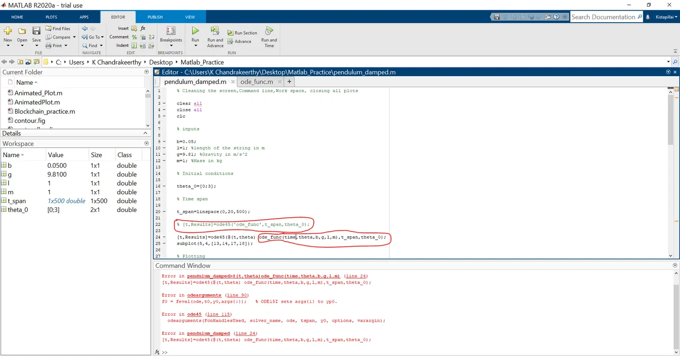
The ode45, the input parameters not same as given.
Error fixed:
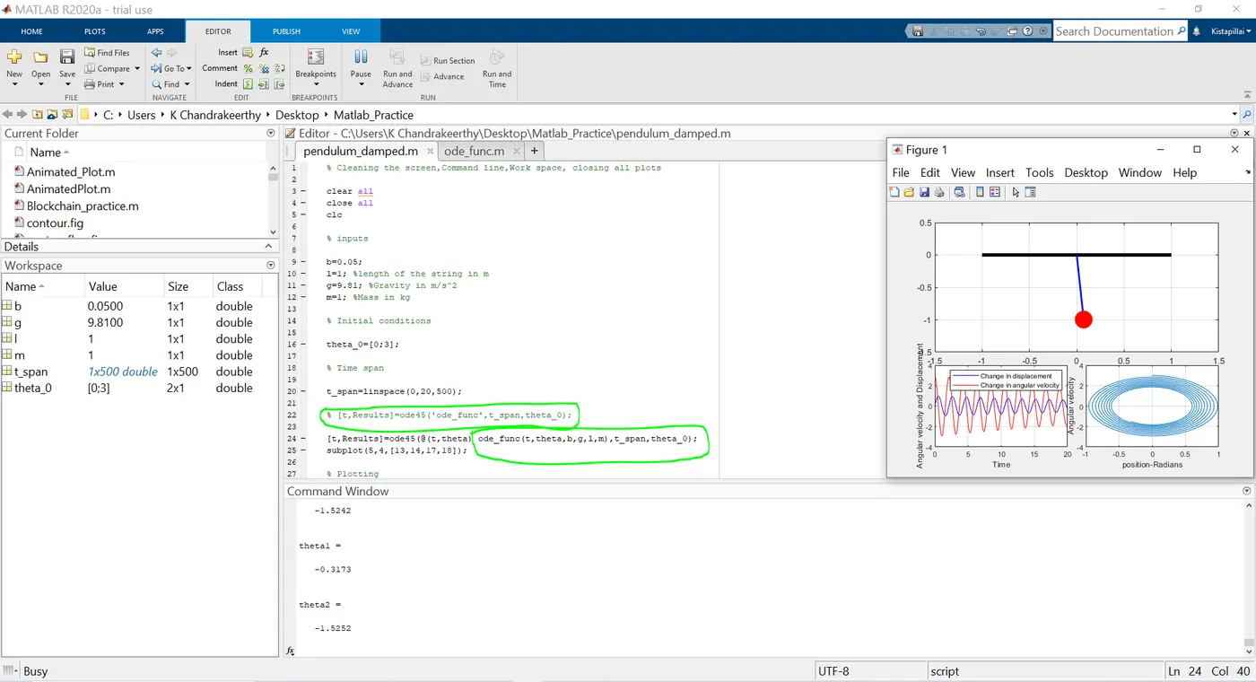
For ode45, the input parameters has been written as per given data.
Errors occured during write a program:
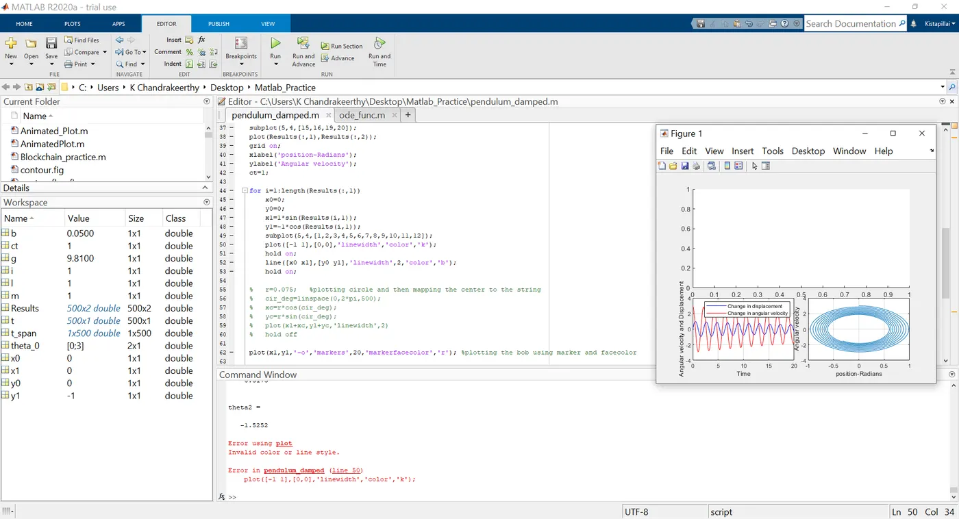
By accidentally forget to write line thickness.
Error fixed:
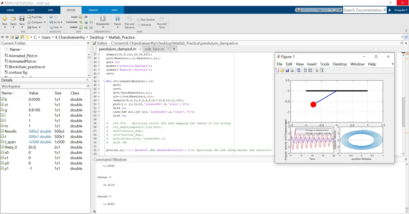
Code corrected back by given the line thickness.
8. Conculation:
The second order ODE is solved, plotted and created as a animation and gif.file. In oder to solving this second order ODE, we can apply the same concepts for higher ODE as well.