Genetic Algorithm

1. Aim:

Understand the concept of Genetic Algorithm. Write a code in MATLAB to optimize the stalagmite function and find the Global maxima of the function. Explain the syntax for Genetic Algorithm in MATLAB.

2. Objectives:

The objective of this project is to optimize the stalagmite function by write a coding program with the help of genetic algorithm in MATLAB as well as explain the concept of genetic algorithm and also explain the syntax of ‘ga’ in MATLAB.

3. Explanation Theory:

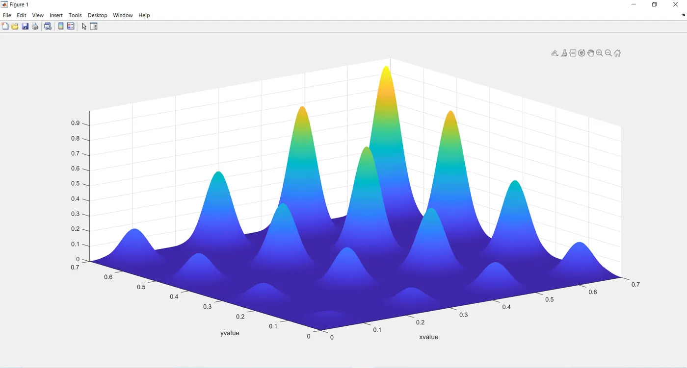
Stalagmite Function: Stalagmites represents the 3D pointed formations arises from the floor. Like cones but may or may not be pointed always. With reference to data here, Stalagmites are the 3D curves formations because of data we gave and it helps finding the threshold value of parameters.

4. History of GA:

As early as 1962, Mr. John Holland’s work on adaptive systems laid the foundations for later developments.

Adaptation in natural and artificial systems book was published in 1975, by J. Holland, his students, and colleagues.

Early to mid-1980s, genetic algorithms were being applied to a broad range of subjects.

In 1992 John Koza has used genetic algorithm to evolve programs to perform certain tasks. He called his method “ Genetic Programming ” (GP).

5. What is Genetic Algorithm:

The genetic algorithm is a method for solving both constrained and unconstrained optimization problems that is based on natural selection, the process that drives biological evolution. The genetic algorithm repeatedly modifies a population of individual solutions. At each step, the genetic algorithm selects individuals at random from the current population to be parents and uses them to produce the children for the next generation. Over successive generations, the population "evolves" toward an optimal solution. You can apply the genetic algorithm to solve a variety of optimization problems that are not well suited for standard optimization algorithms, including problems in which the objective function is discontinuous, nondifferentiable, stochastic, or highly nonlinear. The genetic algorithm can address problems of mixed integer programming, where some components are restricted to be integer valued.

The genetic algorithm uses three main types of rules at each step to create the next generation from the current population:

• Selection rules: select the individuals, called parents, that contribute to the population at the next generation.
• Crossover rules: combine two parents to form children for the next generation.
• Mutation rules: apply random changes to individual parents to form children.

6. Phases of Genetic Algorithm:

Initialization of Population (Coding)

Fitness function

Selection

Reproduction

Convergence (when to stop)

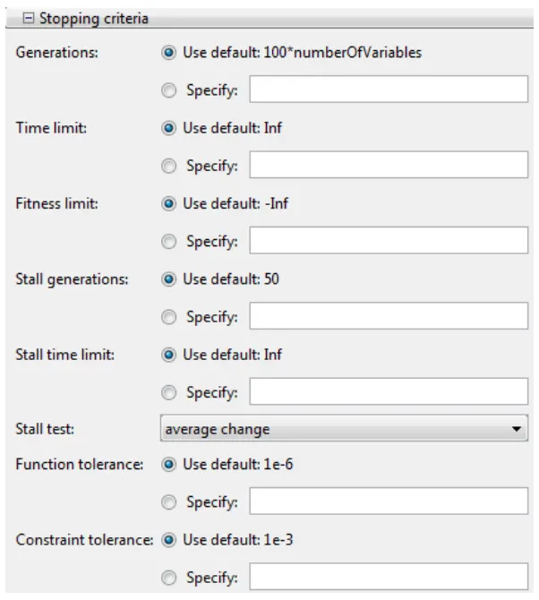
The genetic algorithm uses the following conditions to determine when to stop:

• Generations— The algorithm stops when the number of generations reaches the value of Generations.
• Time limit— The algorithm stops after running for an amount of time in seconds equal to Time limit.
• Fitness limit— The algorithm stops when the value of the fitness function for the best point in the current population is less than or equal to Fitness limit.
• Stall generations— The algorithm stops when the average relative change in the fitness function value over Stall generations is less than Function tolerance.
• Stall time limit— The algorithm stops if there is no improvement in the objective function during an interval of time in seconds equal to Stall time limit.
• Stall test— The stall condition is either average change or geometric weighted. For geometric weighted, the weighting function is 1/2ⁿ, where n is the number of generations prior to the current. Both stall conditions apply to the relative change in the fitness function over Stall generations.
• Function tolerance— The algorithm runs until the average relative change in the fitness function value over Stall generations is less than Function tolerance.
• Constraint tolerance — The Constraint tolerance is not used as stopping criterion. It is used to determine the feasibility with respect to non linear constrains.

The algorithm stops as soon as any one of these condition is met. We can specify the values of these criteria in the Stopping criteria pane in the optimization app. The default values are shown in the pane.

Based on above discussed theory and references, we can write a coding program in MATLAB to optimize the Stalagmite function and find the Global maximum function as follow:

Syntax for 'ga':

x = ga(fun,nvars) - finds a local unconstrained minimum, x, to the objective function, fun. nvars is the dimension (number of design variables) of fun.

x = ga(fun,nvars,A,b) - finds a local minimum x to fun, subject to the linear inequalities A*x ≤ b. ga evaluates the matrix product A*x as if x is transposed (A*x').

x = ga(fun,nvars,A,b,Aeq,beq) - finds a local minimum x to fun, subject to the linear equalities Aeq*x = beq and A*x ≤ b. (Set A=[] and b=[] if no linear inequalities exist.) ga evaluates the matrix product Aeq*x as if x is transposed (Aeq*x').

x = ga(fun,nvars,A,b,Aeq,beq,lb,ub) - defines a set of lower and upper bounds on the design variables, x, so that a solution is found in the range lb ≤ x ≤ ub. (Set Aeq=[] and beq=[] if no linear equalities exist.)

x = ga(fun,nvars,A,b,Aeq,beq,lb,ub,nonlcon) - subjects the minimization to the constraints defined in nonlcon. The function nonlcon accepts x and returns vectors C and Ceq, representing the nonlinear inequalities and equalities respectively. ga minimizes the fun such that C(x) ≤ 0 and Ceq(x) = 0. (Set lb=[] and ub=[] if no bounds exist.)

x = ga(fun,nvars,A,b,Aeq,beq,lb,ub,nonlcon,options) - minimizes with the default optimization parameters replaced by values in options. (Set nonlcon=[] if no nonlinear constraints exist.) Create options using optimoptions.

x = ga(fun,nvars,A,b,[],[],lb,ub,nonlcon,Intcon) - or x = ga(fun,nvars,A,b,[],[],lb,ub,nonlcon,IntCon,options) requires that the variables listed in IntCon take integer values.

x = ga(fun,nvars,A,b,[],[],lb,ub,nonlcon,Intcon,options)

x = ga(problem) - finds the minimum for problem, where problem is a structure.

[x,fval] = ga(___) - for any previous input arguments, also returns fval, the value of the fitness function at x.

[x,fval,exitflag,output] = ga(___) - also returns exitflag, an integer identifying the reason the algorithm terminated, and output, a structure that contains output from each generation and other information about the performance of the algorithm.

[x,fval,exitflag,output,population,scores] = ga(___) - also returns a matrix population, whose rows are the final population, and a vector scores, the scores of the final population.

Syntax for optimization:

option = optimoptions(SolverName)

option = optimoptions(SolverName,Name,Value)

option = optimoptions(oldoptions,Name,Value)

option = optimoptions(SolverNameoldoptions)

option = optimoptions(prob)

option = optimoptions(prob,Name,Value)

Mathematical Equation for Stalagmite Funtion:

`f(x,y) = f1x*f2x*f1y*f2y`

`f1*x=[sin(5.1pix+0.5)]^6`

`f1*y = [sin(5.1piy+0.5)]^6`

`f2,x=exp[-4In(2)(x-0.0667)^2/0.64]`

`f2,y=exp[-4In(2)(y-0.0667)^2/0.64]`

Program for Stalagmite Function:

function [f] = stalagmite(input_vector)
x = input_vector(1);
y = input_vector(2);
f1_x = (sin(5.1*pi*x+0.5)).^6;
f1_y = (sin(5.1*pi*y+0.5)).^6;
f2_x = exp((-4*log(2)*(x-0.667).^2)/0.64);
f2_y = exp((-4*log(2)*(y-0.667).^2)/0.64);

[f] = -(f1_x .* f1_y .* f2_x .* f2_y);

end

Program to optimize stalagmite function and find a global maxima:

clear all
close all
clc

% Defining our search space
x = linspace(0,0.7,200);
y = linspace(0,0.7,200);

% Creating 2 Dimentional mesh
[xx, yy] = meshgrid(x,y);

% Evaluating stalagmite function

for i = 1:length(xx)
    for j = 1:length(yy)
        input_vector(1) = xx(i,j);
        input_vector(2) = yy(i,j);
        f(i,j) = stalagmite(input_vector);
    end
end
    

figure(1)
surfc(xx,yy,-f)
xlabel('xvalue')
ylabel('yvalue')

shading interp

[inputs,fval] = ga(@stalagmite, 2);



% Study 1 - Stastical behaviour
num_case = 70;
tic
for i = 1:num_case
 [inputs,fopt(i)] = ga(@stalagmite, 2);
 xopt(i) = inputs(1);
 yopt(i) = inputs(2);
 
end

study_time_1 = toc;
figure(2)
subplot(2,1,1)
hold on
surfc(xx, yy, -f)
shading interp
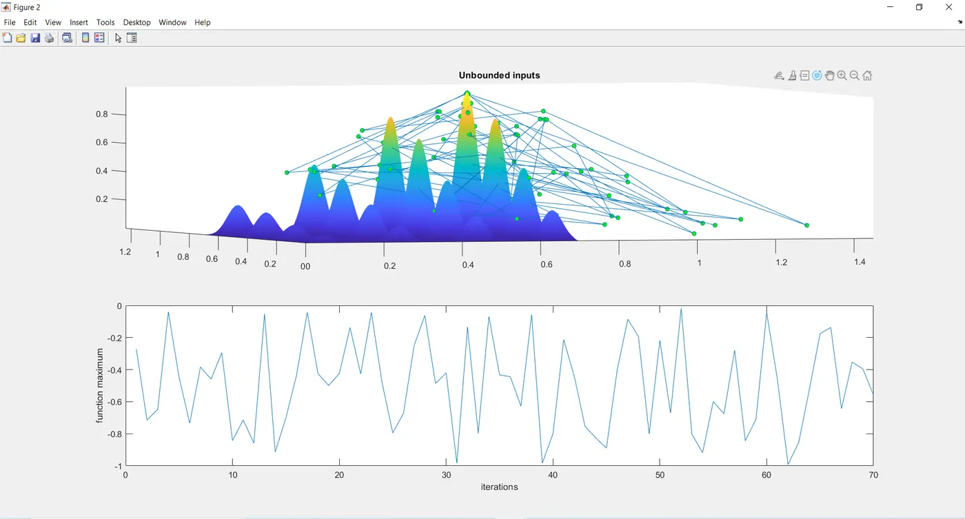
plot3(xopt, yopt, -fopt,'marker','o','markersize',5,'markerfacecolor','g')
title('Unbounded inputs')
subplot(2,1,2)
plot(fopt)
xlabel('iterations')
ylabel('function maximum')

% study 2 Behaviour of Lower and Upper bounded conditions

tic
num_cases = 70;
for i = 1:num_cases
 [inputs,fopt(i)] = ga(@stalagmite, 2,[],[],[],[],[0;0],[1;1]);
 xopt(i) = inputs(1);
 yopt(i) = inputs(2);
 
end

study_time_2 = toc;
figure(3)
subplot(2,1,1)
hold on
surfc(xx,yy,-f)
shading interp
plot3(xopt, yopt, -fopt,'marker','o','markersize',5,'markerfacecolor','g')
title('Lower and Upper bounded inputs')
subplot(2,1,2)
plot(fopt)
xlabel('iterations')
ylabel('function maximum')


% study 3 Behaviour of increasing ga iterations

tic
options = optimoptions('ga');
options = optimoptions(options,'populationsize',400);
for i = 1:num_cases
 [inputs,fopt(i)] = ga(@stalagmite, 2,[],[],[],[],[0;0],[1;1],[],[],options);
 xopt(i) = inputs(1);
 yopt(i) = inputs(2);
 
end

study_time_3 = toc;
figure(4)
subplot(2,1,1)
hold on
surfc(xx,yy,-f)
shading interp
plot3(xopt, yopt, -fopt,'marker','o','markersize',5,'markerfacecolor','g')
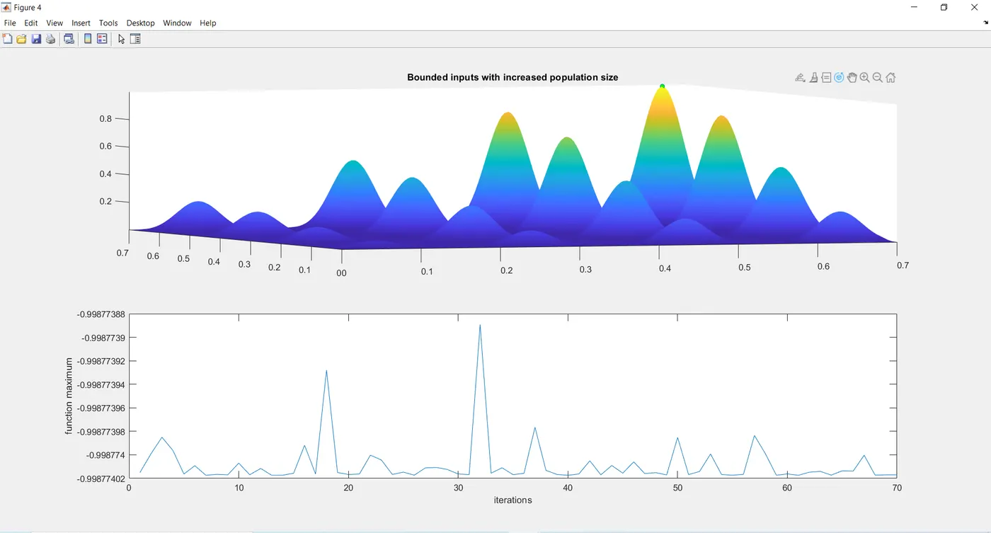
title('Bounded inputs with increased population size')
subplot(2,1,2)
plot(fopt)
xlabel('iterations')
ylabel('function maximum')

Explanation of Matlab codes:

The above written program is for optimize the stalagmite function and find a global maximum of a function.

The code linspace for both axis x and y from 0 to 0.7 and 200 values.

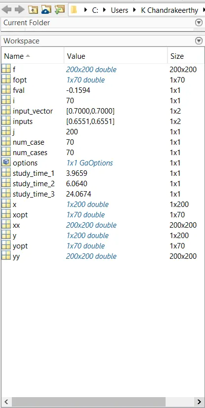
As given the num cases 70, genetic algorithm runs 70 times and calculate study time for 70 iterations.

As genetic algorithm theory, for compilation of this program, 3 stydies are carried out.

% study 1_Satistical behaviour:

In this first study, we calculate the statistical behaviour of stalagmite function by using for loop method, calculate study time with tic toc function and plot as 'x value' and 'y value'.

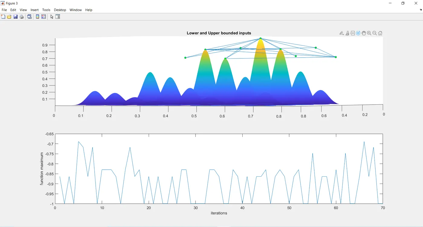
% study 2_Behaviour of upper and lower bounded conditions:

In this second study, we calculate the statistical behaviour of upper and lower bounded conditions with the use of codes:

ga(@stalagmite, 2,[],[],[],[],[0;0],[1;1]),

where, fittnessfcn - stalagmite,

nvars - 2,

[] - Aineq - A matrix for linear inequality constraints

[] - Bineq - B vector for linear inequality constraints

[] - Aeq - A matrix for linear equality constraints

[] - Beq - B vector for linear equality constraints

lb - [0;0] - lower bound on x

ub - [1;1] - upper bound on x

% study 3 Behaviour of increasing ga iterations

In this third study, we calculate the statistical behaviour of increasing the ga iterations. Population size has been increased to 400 and the code as follow:

ga(@stalagmite, 2,[],[],[],[],[0;0],[1;1],[],[],options)

OUTPUT:

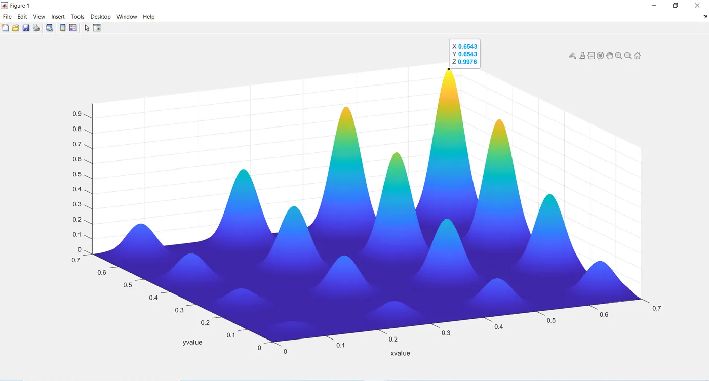
Plotting for stalagmite function:

Plotting for unbounded inputs:

Plotting for lower and upper bounded conditions:

Plotting for increasing ga iterations:

Workspace details:

Conclusion:

From there we came to the conclusion, when multiple number of iterations runs, ga has given the optimum result and the significance of num cases is to check over steadiness of output values of ga whether it gives the same output for all iterations, so that it can undergoes the optimum value, i.e global maximum can be found.

Result:

Thus in my study, the global maximum value has been found as 0.9976 at x = .6543 & y =.6543

References:

1. https://in.mathworks.com/help/gads/ga.html

2. https://www.tutorialspoint.com/genetic_algorithms/genetic_algorithms_crossover.htm

3. https://www.educba.com/what-is-genetic algorithm/