Rankine Cycle Simulator
Aim:
Create a Rankine cycle simulator using Matlab.
Objectives:
- Calculate the state points of the Rankine cycle based on user inputs.
- Calculate the net-work output and back work ratio of the cycle.
- Plot the corresponding T-s and h-s diagrams for a given set of inputs.
Rankine Cycle:
The Rankine cycle is the fundamental operating cycle of all the power plants where an operating fluid is continuously evaporated and condensed. The selection of the operating fluid depends mainly on the available temperature range. In this simulator, the working fluid being used is water.
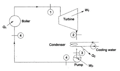
The Rankine cycle operates in the following steps:
1-2: Isentropic Expansion
The vapour is expanded in the turbine, thus producing work which may be converted into electricity. This expansion decreases the temperature and pressure of the vapour and some condensation may occur.
2-3: Constant Pressure Heat Rejection
The vapour-liquid mixture leaving the turbine is condensed at low pressure to become saturated liquid. The pressure vapour is well below atmospheric vapour, approaching the saturation of the operating fluid at the cooling water temperature.
3-4: Isentropic Compression
The working fluid is pumped from low pressure to pressure. The fluid is liquid at this stage due to which the pump requires little input energy. But, because of the low specific volume of the liquid, the pump work is relatively small and is often neglected in TD calculations.
4-1: Constant Pressure Heat Addition
High-pressure liquid enters the boiler from the feed pump and is heated to the saturation temperature. Further addition of energy causes evaporation of the liquid until it is fully converted into saturated steam.
XSteam Library:
Xsteam is a standard libraryto get the steam table datafor the water. It is used to calculate thepoints in betwen the state variables. The library is simple to use and should be stored in the same directory as that of the rankine cycle simulator.
XSteam take 2 or 3 arguments. The first argument must always be the steam table function you want to use. The other arguments are the inputs to that function.
Example: XSteam('h_pt',1,20) Returns the enthalpy of water at 1 bar and 20 degC
Example: XSteam('TSat_p',1) Returns the saturation temperature of water at 1 bar.
Steps to Calculate TD Properties at State Points:
1. State Point 1
- Find `T_(Sat)` from the XSteam library using `P_1`
- Find `H_g` and `S_g` from the XSteam library using P1
- If Tsat > T1 (Saturated Condition)
Calculate H1: `H_1 = H_g`
Calculate S1: `S_1 = S_g` - If Tsat < T1 (Superheated Condition)
Calculate H1: `H_1 = H_g + (C_p)_(vapour)*(T_(Sup) - T_(Sat))`
Calculate S1: `S_1 = S_g + (C_p)_(vapour)*ln(T_(Sup)/T_(Sat))`
2. State Point 2
- `S_2 = S_1` (isentropic process)
- Find `S_g`, `S_f`, `H_g` and `H_f` from the Xsteam library using `P_2`
- If Sg > S2 (Wet)
calculate dryness fraction (x) `x = (S_2 - S_f) / (S_g - S_f)`
calculate H2 `H_2 = H_f + x(H_g - H_f)`
find `T_(sat)` from the XSteam library using P2 `T_2 = T_(sat` - If Sg = S2 (Saturated)
`H_2 = H_g`
Find `T_(sat` from thr XSteam library using `P_2` `T_2 = T_(sat` - If Sg < S2 (Superheated)
`H_2 = H_g + (C_p)_(vapour) * (T_(Sup) - T_(Sat) )`
Calculate T2 from this relation: `S_2 = S_g + (C_p)_(vapour) * ln(T_2/T_(Sat))`
3. State Point 3
- `P_3 = P_2` (isobaric process)
- Find `H_f` from the XSteam library using `P_3`
`H_3 = H_f` - If wet / saturated at State Point 2:
`T_3 = T_2` - If superheated at State Point 2
Find `T_(Sat)` from the XSteam library using P3 `T_3 = T_(Sat`
4. State Point 4
- `P_4 = P_1` (isobaric process)
- Find `V_3` and `S_f` from the XSteam library using P4
- Calculate `H_4` : `H_4 = H_3 + V_3(P_1 - P_2)`
- Calculate `T_4` from this relation `S_4 = S_f - (C_p)_(liquid) * ln(T_4 / T_(Sat))`
- Find `T` from the XSteam library using `P_1` and `H_f` `T_x = T`
- Find `T` from the XSteam library using `P_1` and `H_g` `T_y = T`
- Find `S_f` from the XSteam library using `P_4` `S_x = S_f`
- Find `S_g` from the XSteam library using `P_4` `S_y = S_g`
Program
Below is the program to simulate the Rankine cycle.
The algorithm of the program is as follows:
- Store the input parameters in appropriate variables i.e. P1, T1 and P2.
- Now find the parameters for state point 1 according to the metholodology explained above.
- Subsequently, find the parameters for all state points using the XSteam file and the parameters of previous state points.
- Plot the T-S and H-S diagram using the plot command for all the values of H,T and S at all the respective state points.
- Calculate the cycle parameters like Net Work Done, Efficiency and Back Work Ratio and display them in the command window.
%% Description
%
% This is a program to simulate the Rankine Cycle.
%
%% Outputs
%
% T-S and H-S plots of the Rankine Cycle
%
%% Inputs
%
% 1) Turbine inlet temperature
% 2) Turbine inlet pressure
% 3) Turbine outlet pressure
%
%% Author
%
% Umang Tyagi
% Date of Creation - 19 August 2020
%
%% Program
clear all
close all
clc
fprintf('----------------------------------------------------Rankine Cycle Simulator----------------------------------------------------n')
fprintf('1 - 2 : Isentropic Expansion in the Turbinen')
fprintf('2 - 3 : Constant Pressure Heat Rejection in the Condensern')
fprintf('3 - 4 : Isentropic Compression in the Pumpn')
fprintf('4 - 1 : Constant Presseure Heat Addition by the nn')

%% Parameter Inputs
P1 = input('Enter the Pressure at Turbine Inlet (bar)  :  ');                                  % turbine inlet pressure
T1 = input(['Enter the Temperature at Turbine Inlet ', char(176),'C  :  ']);                   % turbine inlet temperature
P2 = input('Enter the Pressure at Condenser (bar)  :  ');                                      % turbine outlet pressure

%% State Point 1
Tsat_1 = XSteam('Tsat_p',P1);      % saturation temperature at state point 1
Hg_1 = XSteam('hV_p',P1);          % saturated vapour enthalpy at state point 1
Cp_v_1 = XSteam('CpV_p',P1);       % saturated vapour heat capacity at state point 1
Sg_1 = XSteam('sV_p',P1);          % saturated vapour entropy at state point 1

if Tsat_1 > T1       % saturated condition
    H1 = Hg_1;                     % Enthalpy at state point 1
    S1 = Sg_1;                     % Entropy at state point 1
elseif Tsat_1 < T1   % superheated condition
    H1 = Hg_1 + Cp_v_1 * (T1 - Tsat_1);
    S1 = Sg_1 + Cp_v_1 * log(T1/Tsat_1);
end

%% State Point 2
S2 = S1;                           % Entropy at state point 2
Sg_2 = XSteam('sV_p',P2);          % saturated vapour entropy at state point 2
Sf_2 = XSteam('sL_p',P2);          % saturate liquid entropy at state point 2
Hg_2 = XSteam('hV_p',P2);          % saturated vapour enthalpy at state point 2
Hf_2 = XSteam('hL_p',P2);          % saturated liquid enthalpy at state point 2
Tsat_2 = XSteam('Tsat_p',P2);      % saturation temperature at state point 2
Cp_v_2 = XSteam('CpV_p',P2);       % saturated vapour heat capacity at state point 2

if Sg_2 > S2        % wet region
    wet = true;
    x = (S2 - Sf_2)/ (Sg_2 - Sf_2);                % dryness fraction
    H2 = Hf_2 + x*(Hg_2 - Hf_2);                   % Enthalpy at state point 2
    T2 = Tsat_2;                                   % Temperature at state point 2
elseif Sg == S2      % saturation region
    saturated = true;
    H2 = Hg_2;
    T2 = Tsat_2;
else                % superheated region
    superheated  = true;
    T2 = exp((S2 - Sg_2)/ Cp_v_2) * Tsat_2;
    H2 = Hg_2 + Cp_v_2 * (T2 - Tsat_2);
end

%% State point 3
P3 = P2;                              % Pressure at state point 3
V3 = XSteam('vL_p',P3);               % saturated liquid volume at state point 3
Hf_3 = XSteam('hL_p',P3);             % saturated liquid enthalpy at state point 3
Sf_3 = XSteam('sL_p',P3);             % saturated liquid entropy at state point 3
Tsat_3 = XSteam('Tsat_p',P3);         % saturation temperature at state point 3

if wet | saturated      % state point 2's condition was 'wet' or 'saturated'
    T3 = T2;                          % Temperature at state point 3
elseif superheated      % state point 2's condition was 'superheated'
    T3 = Tsat_3;
end

H3 = Hf_3;                            % Enthalpy at state point 3
S3 = Sf_3;                            % Entropy at state point 3

%% State Point 4
P4 = P1;                                   % Pressure at state point 4
S4 = S3;                                   % Entropy at state point 4
Sf_4 = XSteam('sL_p',P4);                  % saturated liquid entropy at state point 4
Sv_4 = XSteam('sV_p',P4);
Hf_4 = XSteam('hL_p',P4);                  % saturated liquid enthalpy at state point 4
Hg_4 = XSteam('hV_p',P4);                  % saturated vapour enthalpy at state point 4
Tsat_4 = XSteam('Tsat_p',P4);              % saturation temperature at state point 4
Cp_l_4 = XSteam('CpL_p',P4);               % saturated liquid heat capacity at state point 4

H4 = H3 + V3*(P1 - P2);                        % Enthalpy at state point 4
T4 = logninv((Sf_4 - S4)/Cp_l_4) * Tsat_4;     % Temperature at state point 4

Tx = XSteam('T_ph',P1,Hf_4);                 % temperature at point x
Ty = XSteam('T_ph',P1,Hg_4);                 % temperature at point y
Sx = Sf_4;
Sy = Sv_4;

%% Work Done and Efficiency Calculation
W_T = H1 - H2;                                 % Work done by turbine
W_P = H4 - H3;                                 % Work done on pump
W_Net = W_T - W_P;                             % Net Work Done
Q1 = H1 - H4;                                  % Heat added to the boiler
Eff = W_Net/Q1 * 100;                          % Efficiency of cycle
BWR = abs(W_P/W_T);                            % back work ratio
%% Plotting

% 1)  T-S Diagram

figure(1)
plot([S1 S2 S3 S4 Sx Sy S1],[T1 T2 T3 T4 Tx Ty T1],'linewidth',1,'color','r');  % plotting the t-s diagram
xlabel('Entropy (kJ/kgK) ')                                                     % labelling axes
ylabel(['Temperature (',char(176),'C)'])
title('t-s diagram')
text(S1,T1,' 1')                                                                % adding reference points on the plot
text(S2,T2,' 2')
text(S3,T3,{'', '3'})
text(S4,T4,{'4',' '})


% 2) H-S Diagram

figure(2)
plot([S1 S2 S3 S4 S1],[H1 H2 H3 H4 H1],'linewidth',1,'color','b')               % plotting the h-s diagram
xlabel('Entropy (kJ/kgK) ')                                                     % labelling the axes
ylabel('Enthalpy (kJ/kg)')
title('h-s diagram')
text(S1,H1,' 1')                                                                % adding reference points on the plot
text(S2,H2,' 2')
text(S3,H3,{'','3'})
text(S4,H4,{'4','',''})

%% Displaying Result
S = [S1 S2 S3 S4];                   % combining result values for reducing code length
T = [T1 T2 T3 T4];
H = [H1 H2 H3 H4];
P = [P1 P2 P3 P4];
fprintf('                                                                   RESULTn')
for i = 1:4
    % printing all 4 result values on all 4 state points, one by one
    fprintf('At State Point %dn',i)
    fprintf('P%d : %f barn',i,P(i))
    fprintf('T%d : %f deg Cn',i,T(i))
    fprintf('H%d : %f kJ/kgn',i,H(i))
    fprintf('S%d : %f kJ/kgKnn',i,P(i))
end

% printing work done, efficiency and back work ratio
fprintf('Work Done by Turbine  : %f kJ/kgn',W_T)
fprintf('Work Done on Pump     : %f kJ/kgn',W_P)
fprintf('Net Work Output           : %f kJ/kgn',W_Net)
fprintf('Efficiency of Cycle         : %fn',Eff)
fprintf('Back Work Ratio           : %fn',BWR)
Output:
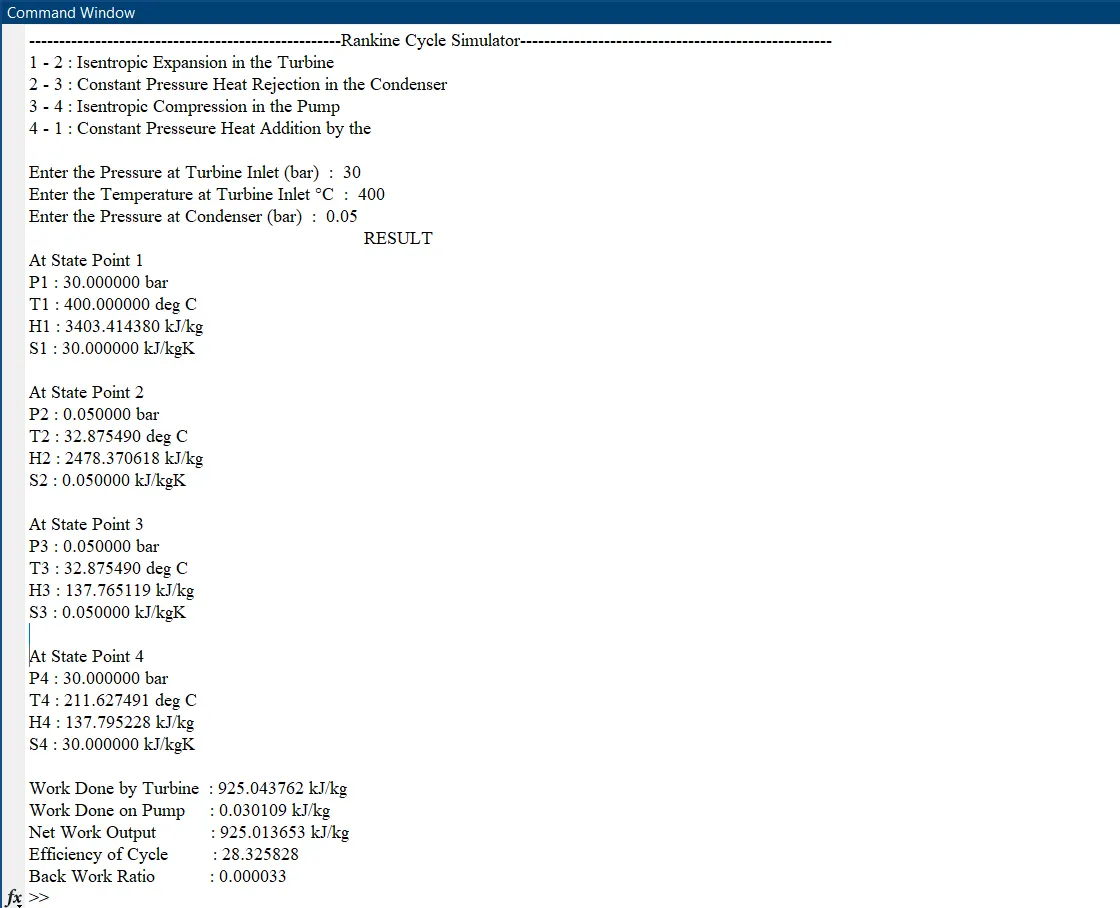
- After running the program, output appears in the command window in which we have to provide the input parameters P1, P2 and T1.

- Here is the screenshot of the final output displayed in the command window after successfully running the program.
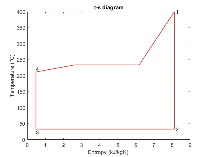
3. Below is the T_S diagram of the above simulated rankine cycle:
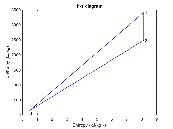
4. Below is the H-S diagram of the above simulated Rankine cycle:
Conclusion:
- The theoretical T-S diagram differs from the practical T-S diagram in such a way that the process 4-1 i.e. Constant Pressure Heat Addition process is a line segment of certain significant length in the theoretical diagram whereas in the practical diagram it only appears as a point.
- This happens because in practical application there is only a slight rise in the temperature which is almost negligible.