Project 2 - Rankine Cycle Simulator

Question

Understand the concept of the Rankine Cycle by referring to the standard thermal engineering textbook.

• Create a Rankine Cycle Stimulator using MATLAB.
  
  
• The code should calculate the state points of the Rankine Cycle (any of your choice) based on user inputs.
  
  
• Then, plot the corresponding T-s and h-s plots for a given set of inputs. Title and axes labels are necessary, while legends could be used.
  
  
• The presentation of your code will be taken into consideration while grading. Labelling sections of your code using comments is appreciated.
  
  
• Attach a report explaining the working of a Rankine Cycle Stimulator and your research.
  
  

The link for the standard Xstream library to get the s is given below. It must be used to calculate the points in between the state variables.

Click here to download the Xsteam Library.

Required Inputs:

1. Turbine Inlet temperature = 400° C
   
   
2. Turbine Inlet Pressure = 30 bars
   
   
3. Turbine Outlet Pressure = 0.05 bars = Condenser Inlet Pressure

Calculate the following,

1. Net work output
   
   
2. Back work ratio.
   
   

Answers

Rankine Cycle

1. History Of The Rankine Cycle

The Rankine cycle is the fundamental operating cycle used by all power plants today. It is a cycle in which all the processes to produce work are reversible and the operating fluid undergoes a continuous cycle of evaporation & condensation.

William John Macquorn Rankine, a Scottish Engineer, continued his study and developed a complete theory of the heat engines along with the steam engine during 1859. The Rankine cycle was named after him honouring his contribution to this subject.

2. What Is Rankine Cycle

The Rankine cycle is an ideal thermodynamic cycle involving a constant-pressure heat engine that converts heat into mechanical work. The heat is supplied externally in this cycle in a closed loop, which uses either water or any other organic fluids (Pentane or Toluene) as a working fluid.

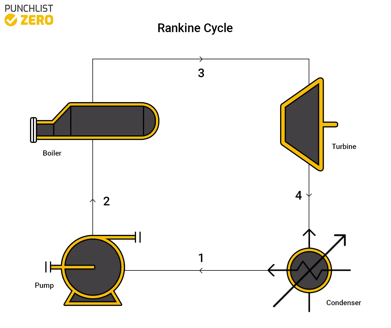
Fig 1: Rankine Cycle Representation

The Rankine cycle is a theoretical cycle on which the power plants work. This cycle, which is the basic principle of Steam turbines, is also known as a modified Carnot cycle. The Carnot cycle is a thermodynamic cycle that has maximum efficiency.

The drawbacks of the Carnot engine like its difficulty to operate practically or to work with superheated steam are overcome by this cycle.

3. Components Of the Rankine Cycle

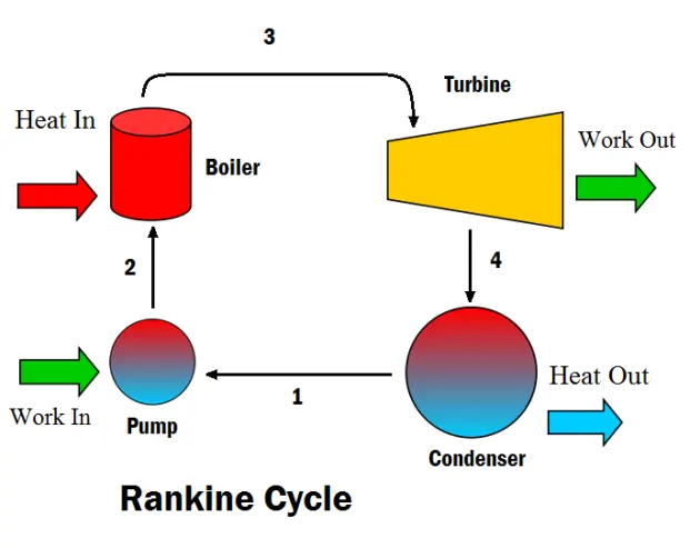
Fig 2: Components Of Rankine Cyclce

A Rankine Cycle consists of four major components as shown in the above figure.

1. Pump :
   They can be centrifugal pumps in industrial applications. Water as saturated liquid enters the pump and is compressed.
   
   
2. Boiler :
   Boilers are generally heat exchangers as in thermal power plants. The compressed liquid enters the boiler to be converted to superheated steam.
   
   
3. Turbines :
   Turbines or steam turbines are machines that use pressurised steam to produce mechanical work. The superheated steam entering the turbine expands and rotates the shaft to produce work which generates electricity.
   
   
4. Condenser :
   The condenser has a set of tubes with a cooling medium surrounding it. The cooling medium may be air or water depending upon the placement of the power plant. Steam, in a saturated liquid-vapour state, is condensed at constant pressure and the heat is rejected to a cooling medium.

4. Working Of Rankine Cycle

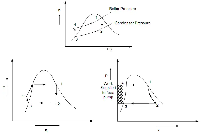
Fig 3: P-V, T-s And h-s Diagram Of Rankine Cycle

1. Process 1-2:
   The working fluid (saturated liquid) entering the pump, is pumped from a low to high pressure. The input energy is needed at this stage. This is also known as isentropic compression
   
   
   
2. Process 2-3:
   Liquid at a high pressure entering the boiler is heated by an external heat source at a constant pressure. The liquid is converted to dry saturated steam by constant pressure heat addition in the boiler.
   
   
3. Process 3-4:
   The dry saturated steam from the boiler expands as it enters the turbine. It is also known as isentropic expansion. Due to this, the temperature and pressure of the steam decrease.
   
   
4. Process 4-1:
   The wet vapour entering the condenser at this stage is condensed at a constant pressure. It is then converted to saturated liquid. This process is also known as constant pressure heat rejection in the condenser. This saturated liquid is again circulated back to the pump, and the cycle continues. The heat rejected or the exhaust heat after the final stage is represented as `Q_(out)`.
   
   
   

5. Efficiency Of The Rankine Cycle

Let us consider these terms that are essential to calculate the efficiency of the cycle.

• `Q`= Rate of heat flow in the system (towards or away)
  
  
• `W_T` = Mechanical work done by the turbine
  
  
• `W_P` = Mechanical work done by the pump
  
  
• `h_1, h_2, h_3 and h_4`= Specific enthalpies of water at states 1, 2, 3, and 4 respectively referring to the T-s diagram
  
  
• `h_f` = Specific enthalpy of water = h (In this case)`

Applying steady flow energy equation (SFEE) to pump, boiler, turbine, and condenser,

• For Pump:
  `h_2+W_P=h_1`
  
  `W_P=h_2-h_1`
  
  
• For Boiler:
  `h_2+Q_("in")=h_3`
  
  `Q_("in")=h_3-h_2`
  
  
  
• For Turbine:
  
  `h_3=W_T+h_4`
  
  `W_T= h_3-h_4`
  
  
• For Condensor:
  
  `h_4=Q_("out")+h_1`
  
  `Q_("out")=h_4-h_1`

So, the Rankine cycle efficiency with the pump is given as


`eta_("Rankine") = W_("net")/(Q_("in"))`

`=(W_T-W_P)/(Q_("in"))`

`=((h_3-h_4)-(h_2-h_1))/(h_3-h_2)`


The Rankine cycle efficiency without the pump is given as

`eta_("Rankine") = 1-Q_("in")/(Q_("out"))`

`1-(h_4-h_1)/(h_3-h_2)`

6. Net Work Output Of The Rankine Cycle

• It is defined as the difference between the work done by the fluid in the turbine (during expansion) and work done on the fluid (during compression).
  
  
• Mathematically, the net work output can be expressed as the area enclosed by the cycle curve on a P-V diagram.
  
  
• Ideally, the pump and turbine in the Rankine cycle would be isentropic, meaning they generate no entropy and maximize the net work output. However, in real-world systems, there are losses due to friction and other factors.

The net work output of the Rankine Cycle is given by

`"Net Work Output" = W_T-W_P`

7. Back Work Ratio (BWR) Of The Rankine Cycle

• Back work ratio (BWR) is a crucial parameter that provides insights into the efficiency and performance of turbines.
  
  
• Specifically, it measures the amount of work required to operate a turbine compared to the work it produces. In gas or steam turbines, the BWR represents the portion of the work output that is used to drive the compressor or pump.
  
  
• This work is essential to maintain the required pressure ratio and ensure continuous turbine operation.
  
  
• A high BWR indicates that a significant portion of the turbine's power output drives the compressor or pump, resulting in lower overall efficiency.
  
  
• Conversely, a lower BWR signifies that a smaller proportion of the power output is consumed by these components, leading to higher efficiency.
  
  

The formula for BWR,
`"BWR"= ("Work Input"-"Work Output")/"Work Output"`

Where Work input refers to the amount of work required to operate the turbine. It includes the work needed to drive the compressor or pump, as well as any other external work input. Work output represents the actual work produced by the turbine. It is the net power output available for useful work, such as generating electricity or driving machinery.

Factors affecting BWR included

• Turbine Efficiency
  
  
• Compressor Efficiency
  
  
• Pressure Ratio
  
  
• Isentropic Efficiency

8. Types Of The Rankine Cycle

The thermodynamic efficiency of the Rankine cycle can be increased by increasing the heat input to the cycle. This can be done by increasing the temperature to change the phase of steam to superheated steam. There are numerous variations like this that attempt to increase the thermodynamic efficiency of the cycle.

Below are some of the cycles designed to increase the thermal efficiency of the cycle.

1. Rankine Cycle with Reheat

Reheating removes the moisture carried by the steam during the final stages of the expansion process in the cycle. With this cycle design, the steam turbines are kept in series to perform the work. Here is a brief on how this cycle works.

1. The high-pressure steam from the boiler enters the first turbine.

2. The steam is passed to the boiler and reheated again.

3. The second turbine is at low pressure to which this reheated steam flows.

The purpose of the Rankine cycle with reheat is to increase the average temperature of the steam in the cycle. Reheating the steam through another stage improves the efficiency of the cycle only half as much as the preceding stage.

2. Regenerative Rankine Cycle

In this cycle, the subcooled liquid from the condenser is heated by the steam trapped in the hot portion of the cycle using a regenerator. This process is mixed with a fluid to convert it to a saturated liquid. Thus, the process is known as ‘Regeneration’, called the ‘regenerative Rankine cycle’.

The regeneration process increases the heat input temperature of the cycle by eliminating the heat addition from the boiler that usually exists in a normal Rankine cycle. As the heat flow into the cycle occurs at a high temperature, the efficiency of the cycle is increased.

3. Organic Rankine Cycle

The organic Rankine cycle, also known as ORC, is a thermodynamic cycle that uses organic fluids like toluene or pentane instead of water and steam. These fluids have a high molecular mass with a higher vaporization temperature than water. It allows heat extraction from a low-temperature source like a solar pond, biomass combustion, or geothermal heat.

4. Supercritical Rankine Cycle

In a supercritical Rankine cycle, the heat is transferred to a high-pressure supercritical fluid, which is then converted to a supercritical phase. Fluid in this phase is sent to a turbine where it expands and helps to generate power. The steam utilised is sent back to be condensed into a liquid and recycled back through the cycle. A supercritical fluid, commonly known as SCF, is a fluid at a temperature and pressure above its critical point. This is the point where liquid and gas do not co-exist. These fluids are found on Earth by black smokers (a type of hydrothermal vent).

9. Applications Of The Rankine Cycle

1. The Rankine cycle with reheating is used in power plants working on fluids at supercritical pressure to generate power.
   
   
2. The regenerative Rankine cycle with a small variation is currently used in thermal power stations like nuclear power plants.
   
   
3. ORC is utilized in various industries like waste heat recovery plants, Biomass power plants, Geothermal power plants, Solar thermal power plants, and Wind-thermal energy stations.
   
   
4. The supercritical Rankine cycles are used in medium power applications like supercritical power plants

10. Matlab Code

The explanation of the syntax of Matlab code is given below.

• With the help of the command 'fprintf', the introduction and the details of the different variables are displayed on the command window.
  
  
  
• Assign the value of turbine I/L pressure or boiler outlet pressure (P1), the value of condenser I/L pressure or turbine O/L pressure (P2) the value of turbine I/L temperature or boiler O/L temperature as user inputs.
  
  
• For finding different state properties we used a function called 'XSteam'. By calling the function with suitable functions and variables we can calculate and assign those values to desirable variables. The main functions and their variables are given below.
  
  

  Sl No	Output	Function	Variable 1	Variable 2
  1	Enthalpy	h_pT	Pressure	Temperature
  2	Entropy	s_pT	Pressure	Temperature
  3	Entropy For Saturated Liquid Region	sL_p	Pressure	-
  4	Entropy For Saturated Vapor Region	sV_p	Pressure	-
  5	Enthalpy For Saturated Liquid Region	hL_p	Pressure	-
  6	Enthalpy For Saturated Vapor Region	hV_p	Pressure	-
  7	Enthalpy	h_ps	Pressure	Entropy
  8	Temperature	T_ph	Pressure	Enthalpy
  9	Temperature	T_ps	Pressure	Entropy
  10	Enthalpy For Saturated Liquid Region	sV_T	Temperature	-
  11	Enthalpy For Saturated Gas Region	sL_T	Temperature	-
  12	Enthalpy For Saturated Liquid Region	hV_T	Temperature	-
  13	Enthalpy For Saturated Gas Region	hL_T	Temperature	-

  
  
  
• For state 1, we have T1 and P1. So using Xsteam and its appropriate function find the remaining variables that are needed for the calculations.
  
  
• Find the dryness fraction, so that it gives an idea of how the cycle works and shows the information about their region in the command window.
  
  
• Similarly, find needed variables for remaining states.
  
  
• Please note the state property conditions for different state regions.
  
  
• Using suitable equations, find pump work, turbine work, heat added to the system and heat rejected from the system.
  
  
• Using calculated values, find the total work done, Rankine efficiency, BWR and SSC. Display to the user with appropriate commands.
  
  
• For plotting the T-s curve, initially, we need to illustrate the saturation line. For that, we need to define an array that has a range of 1 to 373.
  
  
• Choose Figure 1 and hold the figure with suitable commands.
  
  
• Define a for loop for finding saturated entropy values for gas and vapour in each element in the array. Close the for loop. It gives every point based on the coordinates of entropy and temperature values.
  
  
• Join each point by selecting a suitable order for each variable. Manage the plot accordingly.
  
  
• Plot every line by simply inputting the x and y coordinates.
• Manage the plot by adjusting colour, line width, and text messages for labelling the points, title and other options.
  
  
• Similarly, for the h-s diagram, we need to create a figure and assign a name to it.
  
  
• Here using for loop, from the array T1, we need to find the saturated enthalpy values for every temperature value. Join the every pomits.
  
  
• Plot every line by using the coordinates. Manage The Plo.
  
  

The Matlab code is given below.

clear
close
clc

% Matlab Code For Rankine Cycle Stimulator
% Download The Xsteam Library To Get The Steam Table Data For Water
% Move The Xsteam File To The Same Directory Where The Main Code Is Saved.


% Showing The Basics For Running The Rankine Cycle Stimulator
fprintf("Welcome To Rankine Cycle Stimulator\n\n")
fprintf("Please Note The Subscripts For Different State Points And Symbols For\n")
fprintf("Corresponding Variables\n\n\n")
fprintf("Subscripts For Different State Point Includes\n\n")
fprintf("1     = Turbine I/L Or  Boiler O/L\n")
fprintf("2     = Condenser I/L Or Turbine O/L\n")
fprintf("3     = Pump I/L Or Condenser O/L\n")
fprintf("4     = Boiler I/L Or Pump O/L\n")
fprintf("f     = For Fluid (Water)\n")
fprintf("g     = For Gas\n")
fprintf("SatL  = For Saturated Liquid\n")   
fprintf("SatV  = For Saturated Vapor\n")
fprintf("Sat   = Saturated State Points\n\n\n")
fprintf("Variables For Different State Properties\n\n")
fprintf("P   = Pressure\n")
fprintf("V   = Volume\n")
fprintf("T   = Temperature\n")
fprintf("H   = Enthalpy\n")
fprintf("S   = Entropy\n")
fprintf("WT  = Turbine Work\n")
fprintf("WP  = Pump Work\n")
fprintf("Qi  = Heat Added To The System\n")
fprintf("Qo  = Heat Rejected From The System\n")
fprintf("SV  = Specific Volume\n\n\n")
fprintf("Thermodynamic Processes\n\n")
fprintf("Process 1-2  : Isentropic Expansion In Turbine\n")
fprintf("Process 2-3  : Constant Pressure Heat Rejection In Condenser\n")
fprintf("Process 3-4  : Isentropic Compression In Pump\n")
fprintf("Process 4-1  : Constant Pressure Heat Addition In Boiler\n")


% Taking Required Variables As User Inputs
P1 = input("Enter The Value Of Turbine I/L Pressure Or Boiler Outlet Pressure (Bar)= ");
P2 = input("Enter The Value Of Condenser I/L Pressure Or Turbine O/L Pressure  (Bar)= ");
T1 = input("Enter The Value Of Turbine I/L Temperature Or Boiler O/L Temperature (C)= ");


% Result Management
fprintf("\n\n\n\n")
fprintf("Answers")



% Calculating Remaining State 1 Properties Using Steam Table
% Enthalpy At State 1 P1 and T1
H1 = XSteam('h_pT',P1,T1);

% Entropy At State 1 From P1 and T1
S1 = XSteam('s_pT',P1,T1);

% Saturated Vapor Entropy And Saturated Liquid Entropy From P1
Sg1 = XSteam('sV_p',P1);
Sf1 = XSteam('sL_p',P1);

% The Difference Between Sg1 and Sf1 Is Given By
Sfg1 = Sg1-Sf1;

% Dryness Fraction From Sfg2, S2 And Sf2
X1 = (S1-Sf1)/(Sfg1);



% Displaying All-State 1 Properties
fprintf("\n\n")
fprintf("1. State Properties For Point 1\n\n")
fprintf('   P1 =  %2.2f Bar\n',P1)
fprintf('   T1 =  %2.2f °C\n',T1)
fprintf('   H1 =  %7.3f KJ/kg\n',H1)
fprintf('   S1 =  %5.3f KJ/kgK\n',S1)


% Using Dryness Fraction X1 For Finding State Condition
fprintf("\n")
fprintf("   State Condition\n\n")
fprintf('   Dryness Fraction , X1 =   %.3f\n',X1)
fprintf("          State 1 Region =   ")
  

% Define An if Loop For Finding State Condition  
if  X1==0
    fprintf("Saturated Liquid Region (Only Liquid)\n")

elseif (0<X1)&&(X1<1)
    fprintf("Wet Steam Region (Liquid + Vapor)\n")

elseif X1==1
    fprintf("Saturated Vapor State (Pure Dry Steam)\n")

else
    fprintf("Super Heated Steam Region\n")
end



% Calculating State 2 Properties Using Steam Table
% Entropy At State 2 From S1
S2=S1;

% Saturated Vapor Entropy And Saturated Liquid Entropy From P2
Sg2 = XSteam('sV_p',P2);
Sf2 = XSteam('sL_p',P2);

% The Difference Between Sg2 and Sf2 Is Given By,
Sfg2 = Sg2-Sf2;

% Dryness Fraction From Sfg2, S2 And Sf2
X2 = (S2-Sf2)/(Sfg2);

% Saturated Vapor Entropy And Saturated Liquid Entropy From P2
Hg2 = XSteam('hV_p',P2);0;
Hf2 = XSteam('hL_p',P2);

% The Difference Between Hg and Hf
Hfg2 = Hg2-Hf2;


% Enthalpy At State Point 2 From X, Hfg And Hf
if S2<Sg2
    H2 = (X2.*Hfg2)+Hf2;
else
    H2 = XSteam('h_ps',P2,S2);
end


% Temperature At State Point 2 From P2 And H2
T2 = XSteam('T_ph',P2,H2);



% Displaying All-State 2 Properties
fprintf("\n\n")
fprintf("2. State Properties For Point 2\n\n")
fprintf('   P2 =  %2.2f Bar\n',P2)
fprintf('   T2 =  %2.2f °C\n',T2)
fprintf('   H2 =  %7.3f KJ/kg\n',H2)
fprintf('   S2 =  %5.3f KJ/kgK\n',S2)


% Using Dryness Fraction X3 For Finding State Condition
fprintf("\n")
fprintf("   State Condition\n\n")
fprintf('   Dryness Fraction , X2 =   %.3f\n',X2)
fprintf("          State 2 Region =   ")


% Define An if Loop For Finding State Condition 
if  X2==0
    fprintf("Saturated Liquid Region (Only Liquid)\n")

elseif (0<X2)&&(X2<1)
    fprintf("Wet Steam Region (Liquid + Vapor)\n")

elseif X2==1
    fprintf("Saturated Vapor State (Pure Dry Steam)\n")

else
    fprintf("Super Heated Steam Region\n")
end


% Calculating State 3 Properties Using Steam Table
% Pressure At State 3 From P2
P3 = P2;

% Enthalpy At State 3 From Hf2
H3 = Hf2;

% Entrpy At State 3 From Sf2
S3 = Sf2;

% Temperature At State 3 From P3 And S3
T3 = XSteam('T_ps',P3,S3);

% Saturated Vapor Entropy And Saturated Liquid Entropy From Sf2 And Sg2
Sg3 = Sg2;
Sf3 = Sf2;

% The Difference Between Sg3 and Sf3 Is Given By,
Sfg3 = Sfg2;

% Dryness Fraction From Sfg3, S3 And Sf3
X3 = (S3-Sf3)/(Sfg3);


% Displaying All-State 3 Properties
fprintf("\n\n")
fprintf("3. State Properties For Point 3\n\n")
fprintf('   P3 =  %2.2f Bar\n',P3)
fprintf('   T3 =  %2.2f °C\n',T3)
fprintf('   H3 =  %7.3f KJ/kg\n',H3)
fprintf('   S3 =  %5.3f KJ/kgK\n',S3)


% Using Dryness Fraction X3 For Finding State Condition
fprintf("\n")
fprintf("   State Condition\n\n")
fprintf('   Dryness Fraction , X3 =   %.3f\n',X3)
fprintf("          State 3 Region =   ")


% Define An if Loop For Finding State Condition 
if  X3==0
    fprintf("Saturated Liquid Region (Only Liquid)\n")

elseif (0<X3)&&(X3<1)
    fprintf("Wet Steam Region (Liquid + Vapor)\n")

elseif X3==1
    fprintf("Saturated Vapor State (Pure Dry Steam)\n")

else
    fprintf("Super Heated Steam Region\n\n")
end



% Calculating State 3i Properties Using Steam Table
% Pressure At State 3i From P1
P3i = P1;

% Entropy At State 3' From S3
S3i = S3;

% Temperature At State 3' From P3i And S3'
T3i = XSteam('T_ps',P3i,S3i);

% Enthalpy At State 3i From P3i And S4
H3i = XSteam('H_ps',P3i,S3i);



% Displaying All State 3i Properties
fprintf("\n\n")
fprintf("4. State Properties For Point 3i\n\n")
fprintf('   P3i =  %2.2f Bar\n',P3i)
fprintf('   T3i =  %2.2f °C\n',T3i)
fprintf('   H3i =  %7.3f KJ/kg\n',H3i)
fprintf('   S3i =  %5.3f KJ/kgK\n',S3i)


% Calculating State 4 Properties Using Steam Table
% Pressure At State 4 From P1
P4 = P1;

% Entropy At State 4 From Sf1
S4 = Sf1;

% Temperature At State 4 From P4 And S4
T4 = XSteam('T_ps',P4,S4);

% Enthalpy At State 4 From P4 And S4
H4 = XSteam('H_ps',P4,S4);

% Saturated Vapor Entropy And Saturated Liquid Entropy From Sf2 And Sg2
Sg4 = Sg1;
Sf4 = Sf1;

% The Difference Between Sg3 and Sf3 Is Given By,
Sfg4 = Sfg1;

% Dryness Fraction From Sfg3, S3 And Sf3
X4 = (S4-Sf4)/(Sfg4);


% Displaying All-State 4 Properties
fprintf("\n\n")
fprintf("5. State Properties For Point 4\n\n")
fprintf('   P4 =  %2.2f Bar\n',P4)
fprintf('   T4 =  %2.2f °C\n',T4)
fprintf('   H4 =  %7.3f KJ/kg\n',H4)
fprintf('   S4 =  %5.3f KJ/kgK\n',S4)


% Using Dryness Fraction X4 For Finding State Condition
fprintf("\n")
fprintf("   State Condition\n\n")
fprintf('   Dryness Fraction , X4 =   %.3f\n',X4)
fprintf("          State 4 Region =   ")


% Define An if Loop For Finding State Condition 
if  X4==0
    fprintf("Saturated Liquid Region (Only Liquid)\n")

elseif (0<X4)&&(X4<1)
    fprintf("Wet Steam Region (Liquid + Vapor)\n")

elseif X4==1
    fprintf("Saturated Vapor State (Pure Dry Steam)\n")

else
    fprintf("Super Heated Steam Region\n")
end


% Calculating State 4i Properties Using Steam Table
% Pressure At State 4i From P1
P4i = P1;

% Entropy At State 4i' From S4i
S4i = Sg1;

% Temperature At State 3' From P3i And S4i'
T4i = XSteam('T_ps',P4i,S4i);

% Enthalpy At State 3i From P3i And S4
H4i = XSteam('H_ps',P4i,S4i);


% Displaying All State 4i Properties
fprintf("\n\n")
fprintf("6. State Properties For Point 4i\n\n")
fprintf('  P4i =  %2.2f Bar\n',P4i)
fprintf('  T4i =  %2.2f °C\n',T4i)
fprintf('  H4i =  %7.3f KJ/kg\n',H4i)
fprintf('  S4i =  %5.3f KJ/kgK\n',S4i)


% Saturated Vapor Entropy And Saturated Liquid Entropy From Sf2 And Sg2
Sg4i = Sg1;
Sf4i = Sf1;

% The Difference Between Sg3 and Sf3 Is Given By,
Sfg4i = Sfg1;

% Dryness Fraction From Sfg3, S3 And Sf3
X4i = (S4i-Sf4i)/(Sfg4i);


% Using Dryness Fraction X4i For Finding State Condition
fprintf("\n")
fprintf("   State Condition\n\n")
fprintf('   Dryness Fraction , X4i =   %.3f\n',X4i)
fprintf("          State 4i Region =   ")


% Define An if Loop For Finding State Condition 
if  X4i==0
    fprintf("Saturated Liquid Region (Only Liquid)\n")

elseif (0<X4i)&&(X4i<1)
    fprintf("Wet Steam Region (Liquid + Vapor)\n")

elseif X4i==1
    fprintf("Saturated Vapor State (Pure Dry Steam)\n")

else
    fprintf("Super Heated Steam Region\n")
end


% Calculating Work Done And Efficiencies Based On SFEE
% Pump Work From H And H3
WP = H4-H3;

% Turbine Work From H1 And H2
WT = H1-H2;

% Calculating Heat Added (Qi) And Heat Rejected (Qo) Based On SFEE
% Heat Added (Qi) From H1 And H4 
Qi = H1-H4;

% Heat Rejected (Qo) From H2 And H3 
Qo = H2-H3;

% Net Work Output Of The System From WT And WP
W_Net = WT-WP;

% The Rankine Efficiency
% Rankine Efficiency With Pump (Eff_Rankine) From W_Net And Qi
Eff_Rankine = (W_Net/Qi)*100;

% Back Work Ratio, BWR 
BWR = WP/WT;

% Specific Steam Conductivity, SSC
SSC = 3600/W_Net;




% Saturation Temperature Corresponding To P1 Or P4
Tsat_1 = XSteam('Tsat_p',P1);
% Saturation Temperature Corresponding To P2 Or P3
Tsat_2 = XSteam('Tsat_p',P2);
% Displaying The Values


% Displaying All Work Done And Efficiencies
fprintf("\n\n\n")
fprintf("Work Done And Efficiencies In The System\n\n")
fprintf('Turbine Work, WT                          =  %.3f KJ/Kg\n',WT)
fprintf('Pump Work, WP                             =  %.3f KJ/Kg\n',WP)
fprintf('Heat Added To The System, Qi              =  %.3f KJ/Kg\n',Qi)
fprintf('Heat Rejected From The System, Qo         =  %.3f KJ/Kg\n',Qo)
fprintf('Total Work Done By The System, W_Net      =  %.3f KJ/Kg\n',W_Net)
fprintf('Rankine Efficiency With Pump, Eff_Rankine =  %.3f Percent\n',Eff_Rankine)
fprintf('Back Work Ratio, BWR                      =  %.3f \n',BWR)
fprintf('Specific Steam Conductivity, SSC          =  %.3f KJ/Kg\n',SSC)


% Plotting Temperature Vs Entropy (T-s) Curve
% Creating An Array_T1, With 0 to 373 With 373 Elements 
Array_T1 = linspace(1,373,373);

% Assigning Figure
figure(1)
hold on

% Plotting Saturation Curve
% Initiating FOR Loop For The Length Of T1 For Plotting Saturation Points
for i = 1:length(Array_T1)

    % Finding Saturated Vapor Entropy For Every Temperature In 'Array_T1' And For Each Temperature Value
    S_SatV(i) = XSteam('sV_T',Array_T1(i));
   
    % Finding And Plotting Saturated Liquid Entropy For Every Temperature In 'Array_T1' And Each Temperature Value 
    S_SatL(i) = XSteam('sL_T',Array_T1(i));

end


% Connecting All Saturation Points To Create A Saturation Line
plot([S_SatL S_SatV(373:-1:1)],[Array_T1 Array_T1(373:-1:1)], 'linewidth',1, 'color', 'black')


% Plotting T-s Curve
% Plotting T-s Line Connecting State 1 To State 2
plot([S1 S2],[T1 T2], 'linewidth',2, 'color', 'cyan')

% Plotting T-s Line Connecting State 2 To State 3
plot([S2 S3],[T2 T3], 'linewidth',2, 'color', 'green')

% Plotting T-s Line Connecting State 3 To State 3i
plot([S3 S3i],[T3 T3i], 'linewidth',2, 'color', 'yellow')

% Plotting T-s Line Connecting State 3i To State 4
plot([S3i S4],[T3i T4], 'linewidth',2, 'color', 'red')

% Plotting T-s Line Connecting State 4 To State 4i
plot([S4 S4i],[T4 T4i], 'linewidth',2, 'color', 'red')

% Plotting T-s Line Connecting State 4i To State 1
plot ([S4i S1],[T4i T1], 'linewidth',2, 'color', 'red')


% Managing Plots
xlabel('Entropy (KJ/kgK)');
ylabel('Temperature (°C)')
title 'Temperature Vs Entropy (T-s) Diagram'
text(S1,T1,'State 1')
text(S2,T2,'State 2')
text(S3,T3,'State 3')
text(S3i,T3i,'State 3i','Position',[1 50])
text(S4,T4,'State 4')
text(S4i,T4i,'State 4i')
legend ("Saturation Line", "Isentropic Expansion", "Constant Pressure Heat Rejection", "Isentropic Compression", "Constant Pressure Heat Addition")


% Poltting Enthalpy Vs Entropy (h-s) Curve
% Assigning Figure
figure(2)
hold on

% Plotting Saturation Curve
% Initiating FOR Loop For The Length Of T1
for i =1:length(Array_T1)


    % Finding Saturated Vapor Enthalpy For Every Temperature In 'Array_T1' And For Each Temperature Value
    H_SatV(i) = XSteam('hV_T',Array_T1(i));
   
    % Finding And Plotting Saturated Liquid Enthalpy For Every Temperature In 'Array_T1' And Each Temperature Value 
    H_SatL(i) = XSteam('hL_T',Array_T1(i));
 
end

% Connecting All Saturation Points To Create A Saturation Line
plot([S_SatL S_SatV(373:-1:1)],[H_SatL H_SatV(373:-1:1)], 'linewidth',1, 'color', 'black')

% Plotting h-s Line Connecting State 1 To State 2
plot([S1 S2],[H1 H2], 'linewidth',2, 'color', 'cyan')

% Plotting h-s Line Connecting State 2 To State 3
plot([S2 S3],[H2 H3], 'linewidth',2, 'color', 'green')

% Plotting h-s Line Connecting State 3 To State 3i
plot([S3 S3i],[H3 H3i], 'linewidth',2, 'color', 'yellow')

% Plotting h-s Line Connecting State 3i To State 4
plot([S3i S4],[H3i H4], 'linewidth',2, 'color', 'red')

% Plotting h-s Line Connecting State 4 To State 4i
plot([S4 S4i],[H4 H4i], 'linewidth',2, 'color', 'red')

% Plotting h-s Line Connecting State 4i To State 1
plot([S4i S1],[H4i H1], 'linewidth',2, 'color', 'red')


% Managing Plots
xlabel('Entropy (KJ/kgK)');
ylabel('Enthalpy (KJ/kg)')
title 'Enthalpy Vs Entropy (h-s) Diagram'
text(S1,H1,'State 1')
text(S2,H2,'State 2')
text(S3,H3,'State 3')
text(S3i,H3i,'State 3i','Position',[0.6 500])
text(S4,H4,'State 4')
text(S4i,H4i,'State 4i')
legend ("Saturation Line", "Isentropic Expansion", "Constant Pressure Heat Rejection", "Isentropic Compression", "Constant Pressure Heat Addition")

The information shown in the command window for the following question is given below,

Welcome To Rankine Cycle Stimulator

Please Note The Subscripts For Different State Points And Symbols For
Corresponding Variables


Subscripts For Different State Point Includes

1     = Turbine I/L Or  Boiler O/L
2     = Condenser I/L Or Turbine O/L
3     = Pump I/L Or Condenser O/L
4     = Boiler I/L Or Pump O/L
f     = For Fluid (Water)
g     = For Gas
SatL  = For Saturated Liquid
SatV  = For Saturated Vapor
Sat   = Saturated State Points


Variables For Different State Properties

P   = Pressure
V   = Volume
T   = Temperature
H   = Enthalpy
S   = Entropy
WT  = Turbine Work
WP  = Pump Work
Qi  = Heat Added To The System
Qo  = Heat Rejected From The System
SV  = Specific Volume


Thermodynamic Processes

Process 1-2  : Isentropic Expansion In Turbine
Process 2-3  : Constant Pressure Heat Rejection In Condenser
Process 3-4  : Isentropic Compression In Pump
Process 4-1  : Constant Pressure Heat Addition In Boiler
Enter The Value Of Turbine I/L Pressure Or Boiler Outlet Pressure (Bar)= 30
Enter The Value Of Condenser I/L Pressure Or Turbine O/L Pressure  (Bar)= 0.05
Enter The Value Of Turbine I/L Temperature Or Boiler O/L Temperature (C)= 400




Answers

1. State Properties For Point 1

   P1 =  30.00 Bar
   T1 =  400.00 °C
   H1 =  3231.571 KJ/kg
   S1 =  6.923 KJ/kgK

   State Condition

   Dryness Fraction , X1 =   1.208
          State 1 Region =   Super Heated Steam Region


2. State Properties For Point 2

   P2 =  0.05 Bar
   T2 =  32.88 °C
   H2 =  2110.708 KJ/kg
   S2 =  6.923 KJ/kgK

   State Condition

   Dryness Fraction , X2 =   0.814
          State 2 Region =   Wet Steam Region (Liquid + Vapor)


3. State Properties For Point 3

   P3 =  0.05 Bar
   T3 =  32.87 °C
   H3 =  137.765 KJ/kg
   S3 =  0.476 KJ/kgK

   State Condition

   Dryness Fraction , X3 =   0.000
          State 3 Region =   Saturated Liquid Region (Only Liquid)


4. State Properties For Point 3i

   P3i =  30.00 Bar
   T3i =  32.95 °C
   H3i =  140.762 KJ/kg
   S3i =  0.476 KJ/kgK


5. State Properties For Point 4

   P4 =  30.00 Bar
   T4 =  233.85 °C
   H4 =  1008.329 KJ/kg
   S4 =  2.646 KJ/kgK

   State Condition

   Dryness Fraction , X4 =   0.000
          State 4 Region =   Saturated Liquid Region (Only Liquid)


6. State Properties For Point 4i

  P4i =  30.00 Bar
  T4i =  233.86 °C
  H4i =  2803.265 KJ/kg
  S4i =  6.186 KJ/kgK

   State Condition

   Dryness Fraction , X4i =   1.000
          State 4i Region =   Saturated Vapor State (Pure Dry Steam)



Work Done And Efficinecies In The System

Turbine Work, WT                          =  1120.863 KJ/Kg
Pump Work, WP                             =  870.564 KJ/Kg
Heat Added To The System, Qi              =  2223.242 KJ/Kg
Heat Rejected From The System, Qo         =  1972.943 KJ/Kg
Total Work Done By The System, W_Net      =  250.298 KJ/Kg
Rankine Efficiency With Pump, Eff_Rankine =  11.258 Percent
Back Work Ratio, BWR                      =  0.777 
Specific Steam Conductivity, SSC          =  14.383 KJ/Kg

The T-s and h-s Plot for the following problems are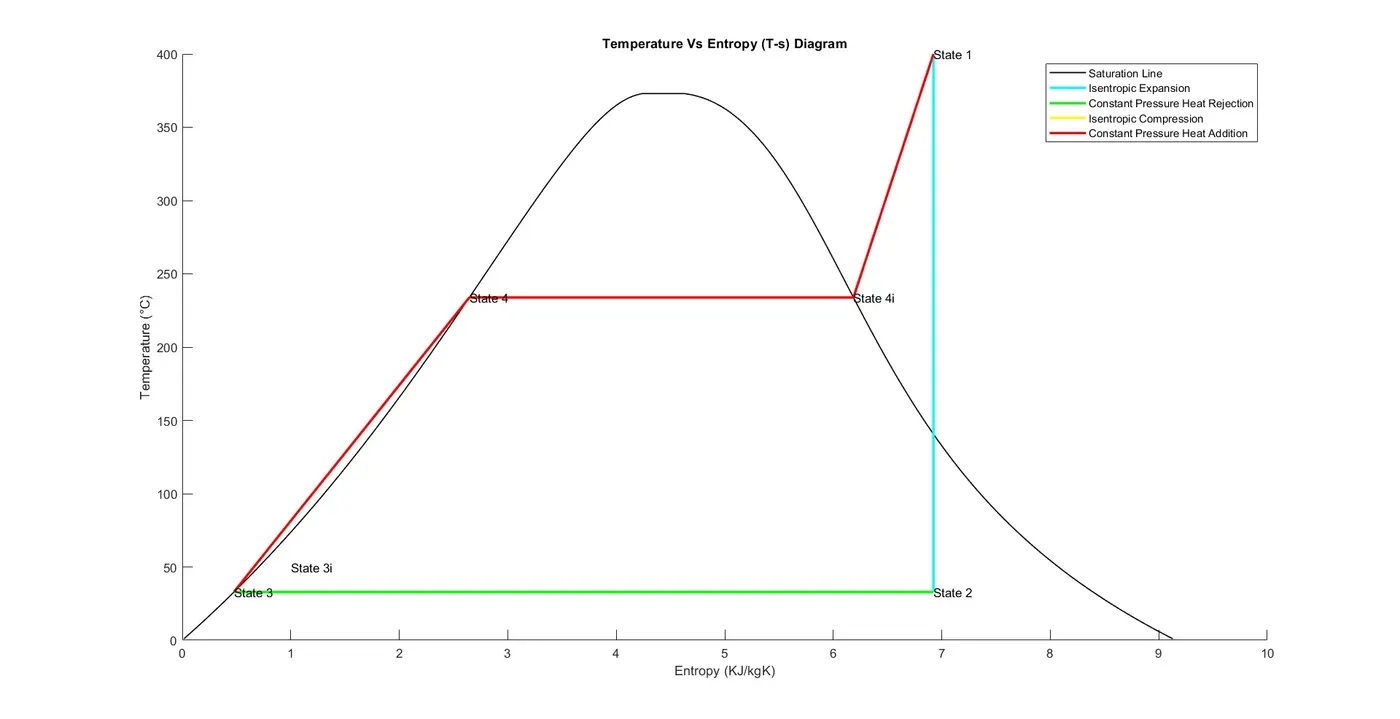

T- s Diagram

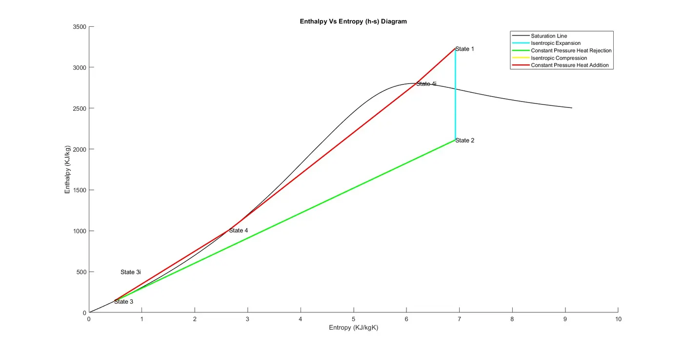
h- s Diagram

11. Errors Faced During The Process

• There are some errors due to a misunderstanding of some codes and values. Other than that the coding process was fine.

References

1. Rankine Cycle: Know Definition, Types, Working Principle & More (testbook.com)