Project 2 - Rankine cycle Simulator
Aim:
To create a Rankine cycle simulator by using MATLAB.
Objective:
- To calculate the state points of the Rankine cycle based on user inputs
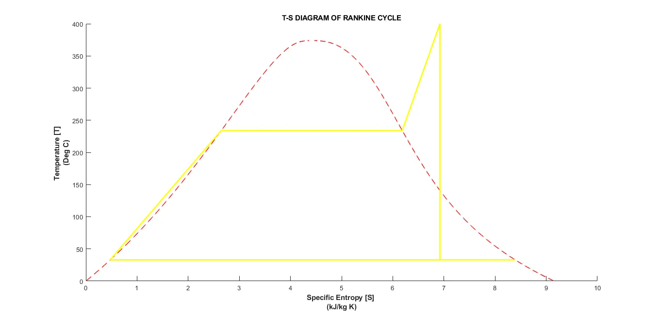
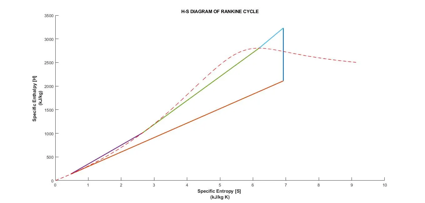
- To plot corresponding T-s and h-s diagrams.
Introduction to the cycle:
The Rankine cycle is an idealized thermodynamic cycle describing the process by which certain heat engines, such as steam turbines or reciprocating steam engines, allow mechanical work to be extracted from a fluid as it moves between a heat source and heat sink.
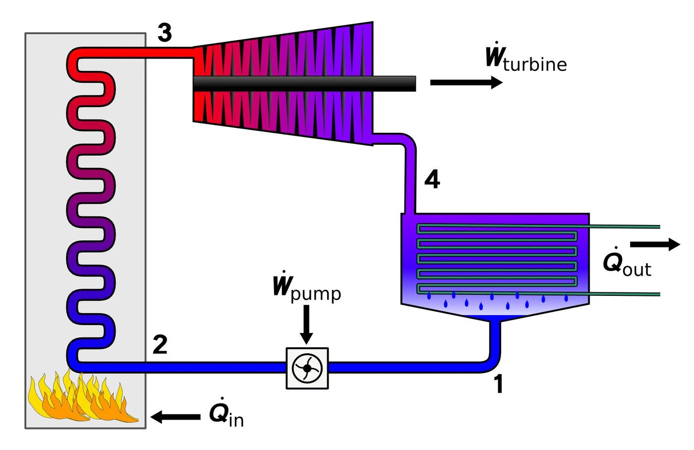
Heat energy is supplied to the system via a boiler where the working fluid (typically water) is converted to a high pressure gaseous state (steam) in order to turn a turbine. After passing over the turbine the fluid is allowed to condense back into a liquid state as waste heat energy is rejected before being returned to boiler, completing the cycle. Friction losses throughout the system are often neglected for the purpose of simplifying calculations as such losses are usually much less significant than thermodynamic losses, especially in larger systems.
The Four process in the Rankine cycle:
There are four processes in the Rankine cycle. The states are identified by numbers (in brown) in the T–s diagram.
- Process 1-2: Isentropic compression in a pump. The working fluid is pushed from low to high pressure in this chamber.
- Process 2-3: Heat addition at constant pressure in the boiler. ...
- Process 3-4: Isentropic expansion in a turbine. ...
- Process 4-1: Heat rejection under constant pressure in a condenser.
In an ideal Rankine cycle the pump and turbine would be isentropic: i.e., the pump and turbine would generate no entropy and would hence maximize the net work output. Processes 1–2 and 3–4 would be represented by vertical lines on the T–s diagram and more closely resemble that of the Carnot cycle. The Rankine cycle shown here prevents the state of the working fluid from ending up in the superheated vapor region after the expansion in the turbine, [1] which reduces the energy removed by the condensers.
The actual vapor power cycle differs from the ideal Rankine cycle because of irreversibilities in the inherent components caused by fluid friction and heat loss to the surroundings; fluid friction causes pressure drops in the boiler, the condenser, and the piping between the components, and as a result the steam leaves the boiler at a lower pressure; heat loss reduces the net work output, thus heat addition to the steam in the boiler is required to maintain the same level of net work output.
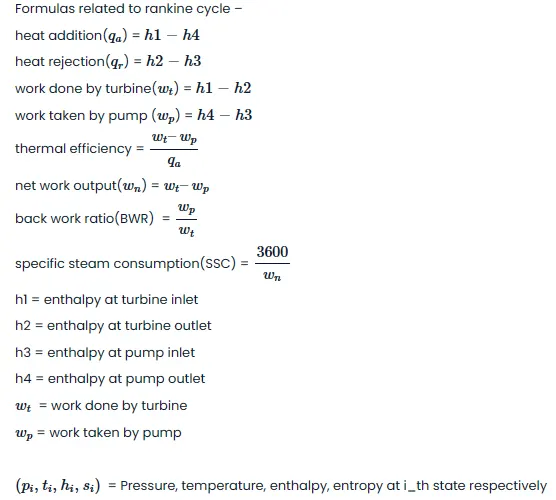
Matlab code:
clear all
close all
clc
�sic Info
fprintf('`s \r\n', 'Rankine Cycle Simulator')
fprintf('%s \n','Process 1-2 is Isentropic Expansion in Turbine')
fprintf('%s \n','Process 2-3 is Constant Pressure Heat Rejection by Condenser')
fprintf('%s \n','Process 3-4 is Isentropic Compression in Pump')
fprintf('%s \r\n','Process 4-1 is Constant Pressure heat Addition by Boiler')
%% INPUTS
p1=input('Enter the pressure at turbine Inlet : ');
t1=input('Enter the temperature at turbine Inlet : ');
p2=input('Enter the pressure at condensor Inlet : ');
%% 1-2 Isentropic Turbine Expansion
h1=XSteam('h_pT',p1,t1);
s1=XSteam('s_pT',p1,t1);
tsat1=XSteam('Tsat_p',p1); %Saturation Temp.at p1
hg1=XSteam('hV_p',p1);
hf1=XSteam('hL_p',p1);
sg1=XSteam('sV_p',p1);
sf1=XSteam('sL_p',p1);
s2=s1;
hf2=XSteam('hL_p',p2);
sf3=XSteam('sL_p',p2);
hg2=XSteam('hV_p',p2);
sg2=XSteam('sV_p',p2);
sfg=sg2-sf3; %entropy of wet region
hfg= hg2-hf2;
if s2 < sg2>
x2=(s2-sf3)/sfg; �lculates the new quality at this point
h2=hf2+x2*hfg; �lculates the new enthalpy
else
x2 = 1; % Quality is max 1
h2 = x2*hg2; �lculates the new enthalpy
end
t2=XSteam('T_ps',p2,s2);
tsat2=XSteam('Tsat_p',p2); %Saturation Temp.at p2
%% 2-3 Isobaric Condenser
p3=p2;
s3=sf3;
h3=hf2;
%% 3-4 Isentropic Pump
s4=s3;
t3=tsat2;
%% 4-1 Isobaric Boiler
p4=p1;
h4=XSteam('h_ps',p4,s4);
t4=XSteam('T_ps',p4,s4);
%% T-S & H-S Diagrams
t= linspace(1,t1,5000);
figure(1)
%axis([1.91984 1.92 157.4 158.3]);
hold on
sl=zeros;
sv=zeros;
hl=zeros;
hv=zeros;
for i=1:length(t)
sl(i)=XSteam('sL_T',t(i));
sv(i)=XSteam('sV_T',t(i));
hl(i)=XSteam('hL_T',t(i));
hv(i)=XSteam('hV_T',t(i));
end
plot(sl,t,'--r','linewidth',1)
plot(sv,t,'--r','linewidth',1)
%% T-S Diagram Animation
for i=s1:s2
a=linspace(s1,s2,100);
b=linspace(t1,t2,100);
curve=animatedline('color','y','linewidth',2);
for j=1:100
x=a(j);
y=b(j);
addpoints(curve,x,y);
pause(0.01) ;
end
end
for i=sg2:s2
a=linspace(s2,sg2,100);
b=linspace(t2,tsat2,100);
curve=animatedline('color','y','linewidth',2);
for j=1:100
x=a(j);
y=b(j);
addpoints(curve,x,y);
pause(0.01) ;
end
end
for i=s3:sg2
a=linspace(sg2,s3,100);
b=linspace(tsat2,t3,100);
curve=animatedline('color','y','linewidth',2);
for j=1:100
x=a(j);
y=b(j);
addpoints(curve,x,y);
pause(0.01) ;
end
end
for i=s3:s4
a=linspace(s3,s4,100);
b=linspace(t3,t4,100);
curve=animatedline('color','y','linewidth',2);
for j=1:100
x=a(j);
y=b(j);
addpoints(curve,x,y);
pause(0.01) ;
end
end
for i=s4:sf1
a=linspace(s4,sf1,100);
b=linspace(t4,tsat1,100);
curve=animatedline('color','y','linewidth',2);
for j=1:100
x=a(j);
y=b(j);
addpoints(curve,x,y);
pause(0.01) ;
end
end
for i=sf1:sg1
a=linspace(sf1,sg1,100);
b=linspace(tsat1,tsat1,100);
curve=animatedline('color','y','linewidth',2);
for j=1:100
x=a(j);
y=b(j);
addpoints(curve,x,y);
pause(0.01) ;
end
end
for i=sg1:s1
a=linspace(sg1,s1,100);
b=linspace(tsat1,t1,100);
curve=animatedline('color','y','linewidth',2);
for j=1:100
x=a(j);
y=b(j);
addpoints(curve,x,y);
pause(0.01) ;
end
end
%
%plot([s1 s2],[t1 t2],'linewidth',2)
%plot([s2 sg2],[t2 tsat2],'linewidth',2)
%plot([sg2 s3],[tsat2 t3],'linewidth',2)
%plot([s3 s4],[t3 t4],'linewidth',2)
%plot([s4 sf1],[t4 tsat1],'linewidth',2)
%plot([sf1 sg1],[tsat1 tsat1],'linewidth',2)
%plot([sg1 s1],[tsat1 t1],'linewidth',2)
xlabel({'Specific Entropy [S] ','(kJ/kg K)'},'FontWeight','bold')
ylabel({'Temperature [T] ','(Deg C)'},'FontWeight','bold')
title('T-S DIAGRAM OF RANKINE CYCLE', 'FontWeight', 'bold');
%% H-S Diagram Animation
figure(2)
hold on
plot([s1 s2],[h1 h2],'linewidth',2)
plot([s2 s3],[h2 h3],'linewidth',2)
plot([s3 s4],[h3 h4],'linewidth',2)
plot([s4 sf1],[h4 hf1],'linewidth',2)
plot([sf1 sg1],[hf1 hg1],'linewidth',2)
plot([sg1 s1],[hg1 h1],'linewidth',2)
plot([sl sv],[hl hv],'--r','linewidth',1)
xlabel({'Specific Entropy [S] ','(kJ/kg K)'},'FontWeight','bold')
ylabel({'Specific Enthalpy [H] ' ,'(kJ/kg)'},'FontWeight','bold')
title('H-S DIAGRAM OF RANKINE CYCLE', 'FontWeight', 'bold');
%�ficiency and Work
Wt=h1-h2;
Wp=h4-h3;
W=Wt-Wp;
qin=h1-h4;
qout=h2-h3;
eff=W*100/qin;
bwr=qin/qout;
%% Display
fprintf('%-60s s \r\n', 'At State Point 1','At State Point 2' )
fprintf('%s %.2f %s ds %.2f %s \n','P1:',p1,'bar','P2:',p2,'bar')
fprintf('%s %.2f %s Us %.2f %s \n','T1:',t1,'deg Celcius','T2:',t2,'deg Celcius')
fprintf('%s %.2f %s `s %.2f %s \n','H1:',h1,'kJ/Kg','H2:',h2,'kJ/Kg')
fprintf('%s %.2f %s as %.2f %s \r\n','S1:',s1,'kJ/Kg K','S2:',s2,'kJ/Kg K')
fprintf('%-60s s \r\n', 'At State Point 3','At State Point 4' )
fprintf('%s %.2f %s ds %.2f %s \n','P3:',p3,'bar','P4:',p4,'bar')
fprintf('%s %.2f %s Us %.2f %s \n','T3:',t3,'deg Celcius','T3:',t4,'deg Celcius')
fprintf('%s %.2f %s `s %.2f %s \n','H3:',h3,'kJ/Kg','H4:',h4,'kJ/Kg')
fprintf('%s %.2f %s `s %.2f %s \r\n','S3:',s3,'kJ/Kg K','S4:',s4,'kJ/Kg K')
fprintf('`s %.2f %s \n','Work Done by Turbine:',Wt,'kJ/Kg')
fprintf('`s %.2f %s \n','Work Done by Pump:',Wp,'kJ/Kg')
fprintf('`s %.2f %s \n','Net Work Done:',W,'kJ/Kg')
fprintf('`s %.2f %s \n','Heat Input in boiler:',qin,'kJ/Kg')
fprintf('`s %.2f %s \n','Heat rejected in Condenser:',qout,'kJ/Kg')
fprintf('`s %.2f \n','Back Work Ratio:',bwr)
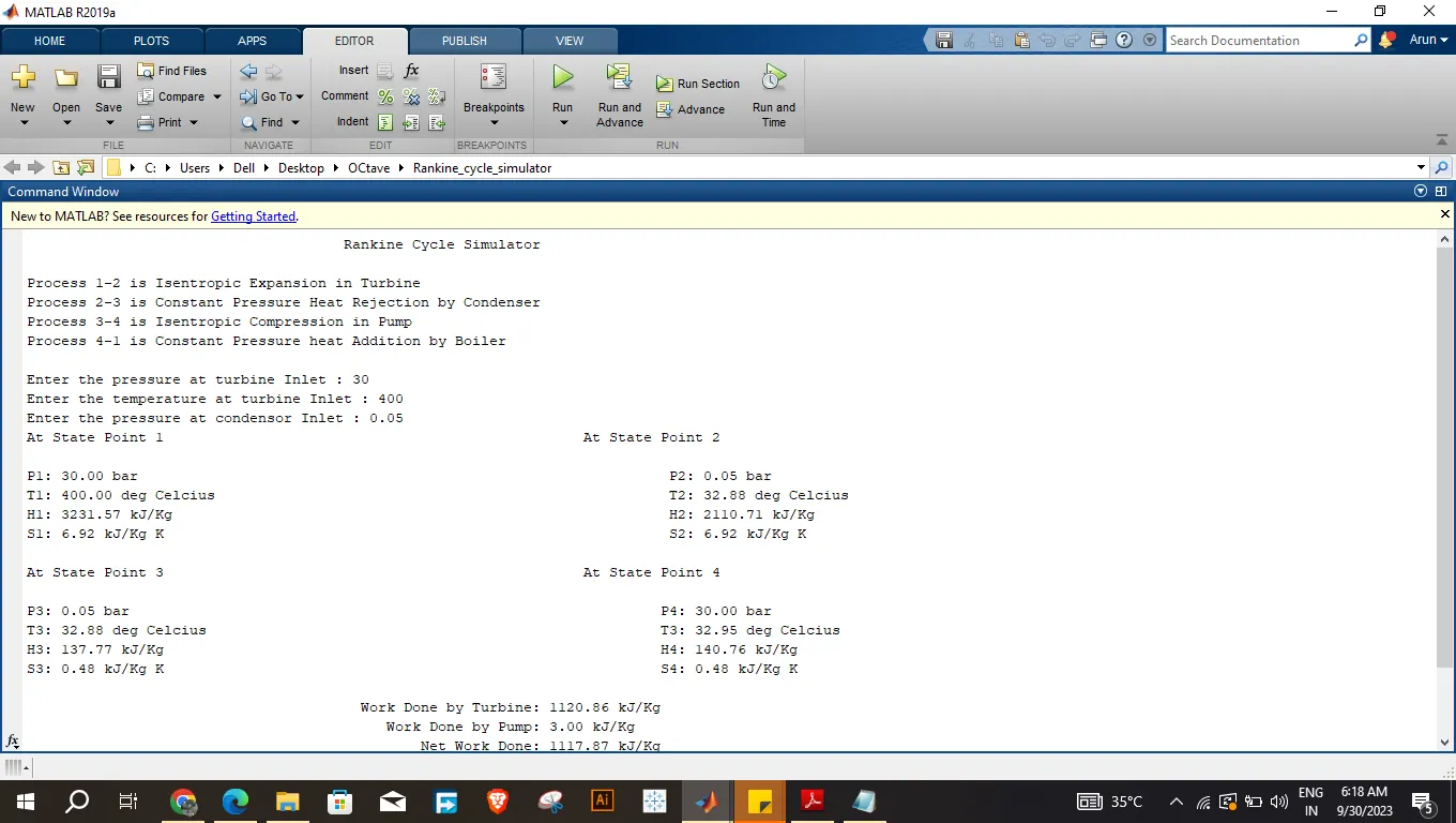
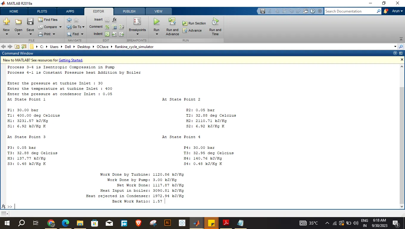
Screenshot of the Matlab command window:
Results:
T-s plot:
h-s plot:
Reference link:
https://en.wikipedia.org/wiki/Rankine_cycle
Rankine Cycle (Steam Turbine) - MATLAB & Simulink - MathWorks India