Project - 2 - Meshing on the suspension Assembly

Aim:

To mesh the given rear suspension model in both 2D and 3D (according to the given quality criteria) after checking for and clearing geometrical errors. Also, to deploy appropriate connections as required between various parts of the assembly after which the model is symmetrically replicated using the reflect tool.

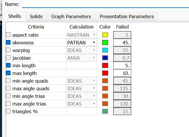
Quality Criteria for Surface Meshing of Tyre and Rim (Element type: Tria) : 

S.No	Quality Criteria	Value
1	Target/Average length	6.5
2	Minimum Length	5
3	Maximum Length	10
4	Skewness	45

 Quality criteria for Surface Meshing of Non Uniform thickness components other than Tyre and Rim (Element type: Tria) :

S.No	Quality Criteria	Value
1	Target/Average length	4
2	Minimum Length	2
3	Maximum Length	6
4	Skewness	45

 Quality Criteria for Volume meshing of all Non Uniform thickness components (Element type: Tetra Elements): 

S.No	Quality Criteria	Value
1	Tet-collapse	0.2

 Quality criteria for Mid surfacing of Uniform thickness part which has thickness less than 5 mm (Element type: Mixed elements) :

S.No	Quality Criteria	Value
1	Target/Average length	4
2	Minimum Length	2
3	Maximum Length	6
4	Aspect	3
5	Warpage	15
6	Skewness	45
7	Jacobian	0.7
8	Minimum Quad Angle	45
9	Maximum Quad Angle	135
10	Minimum  Tria Angle	30
11	Maximum Tria Angle	120

Procedure:

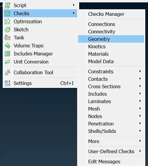
1. The first step is to check the topology of the imported model. In tnis model many components are present because of that we have to check the part one by one. Clear all the single cons and triple cons if any present. The command used is check > geometry.

2. There are many components with different thickness so we done separation of components and set a new Prperty id.

After the creation of new PIds we done the 3Dmeshing and 2Dmesing.

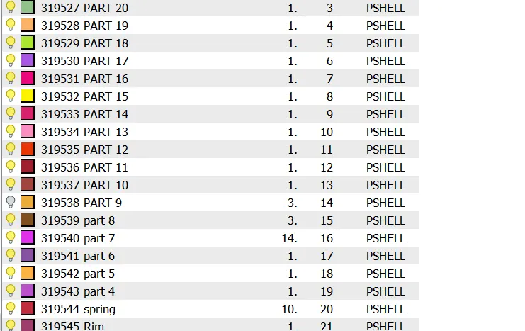
While assigning PIDs, we can midsurface the parts that will require 2D meshing and then assign PIDs to these midsurfaces as well. For midsurfacing, I used the offset tool (Faces > Offset). When activated, it will ask us to select the surfaces to offset. We can select the surfaces on one side of the part. After that, we can assign the offset value (half the thickness). The offset tool will show the direction of the offset in the form of an arrow. If it is in the opposite direction of the required offset, the offset value needs to be in the negatives. If we proceed, the surface will be offset and we will have the option of keeping the parent surfaces.

3. Next is to perform the meshing. Based on the thickness that is less than 5mm we used the 2d meshing and above 5mm we used the solid meshing finally the nonuniform part also carried the solid meshing. Here first started with the volume meshong.

4. For the parts first we have to carried the surface meshing by using the tri as the elements. here we can use either batch meshing or mannual meshing.

The quality criteria for the tyre and rim.

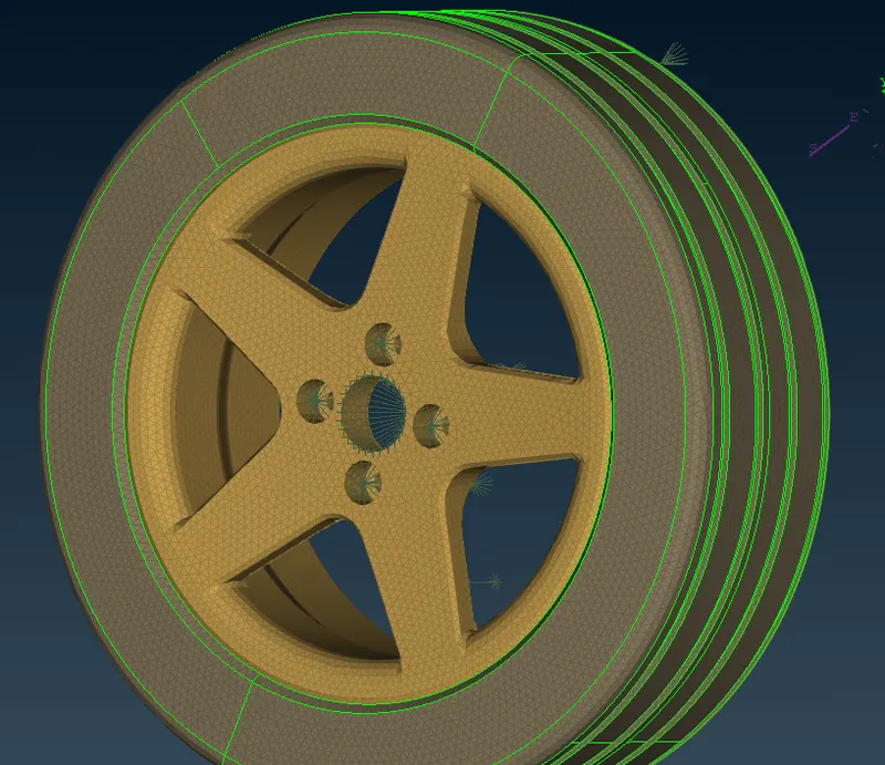
7. We can then start meshing each of the parts as per the mesh requirements (2D Mixed mesh using Mesh Generation > Best from the Mesh module and 2D tria mesh using Mesh Generation > Spot. In the following example, I have started meshing the rim starting from the centre, in an outward direction. After that, we can make use of the reconstruct tool Shell Mesh > Reconstruct)to generate a better mesh if the initial mesh is not satisfactory. If required, the smooth tool Shell Mesh > Smooth can be used as well.

5.After meshing all regions, we can proceed to the next step of assigning volumes manually to each set of closed-shell elements (for volumetric meshing). This is done by using Volumes > Define > Manual and then selecting the regions that comprise a particular volume. Auto automatically detects and defines closed volumes that are selected whereas the manual option lets us define properties for the volume that is to be defined. Either method works here.

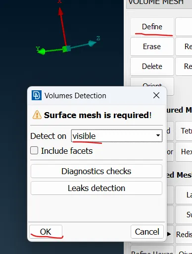
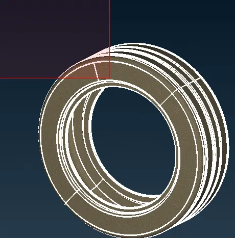
6.After the volume is defined, the list of defined volumes can be accessed from Volumes > List. The volumes that are unmeshed can be 3D meshed by rt. clicking the particular volume and selecting 'remesh' as shown:

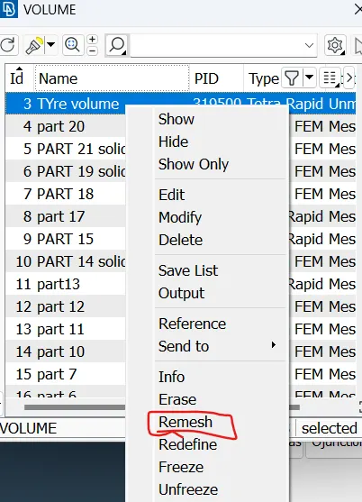
This process is repeated individually for every available volume in the model.

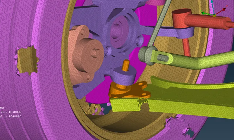
7. After the creation of the volume mesh we have to check for the failed elements which are present. The failed elements are cleared by using the Fix Quality tool from the volume mesh module Improve > Fix Quality.

8. To avoid the  protrusions or depressions on an otherwise flat surface,the MV free tool can be used (Grids > MV Free) which is available in the mesh module. This lets us manually drag particular nodes of the failing element such that the height of the tetra element can be increased. This helps pass the tet collapse criteria. Understandably, to avoid the same problem as in the Fix Quality tool, care should be taken to not move nodes that are on the surface of the component but the ones that are below the surface.

9. After the completion of the 3D meshing we have done the 2d meshing. The parts having a uniform thickness has done with midsurface by the command mid surfaces > skin used here.

 

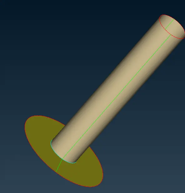
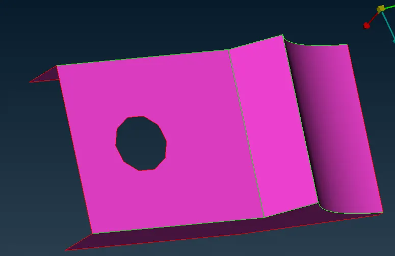
The meshing is carried out after the midsurfacing. The quality criteria which was given in the question particularly for the uniform thickness is maintained. Mixed types of elements is used.

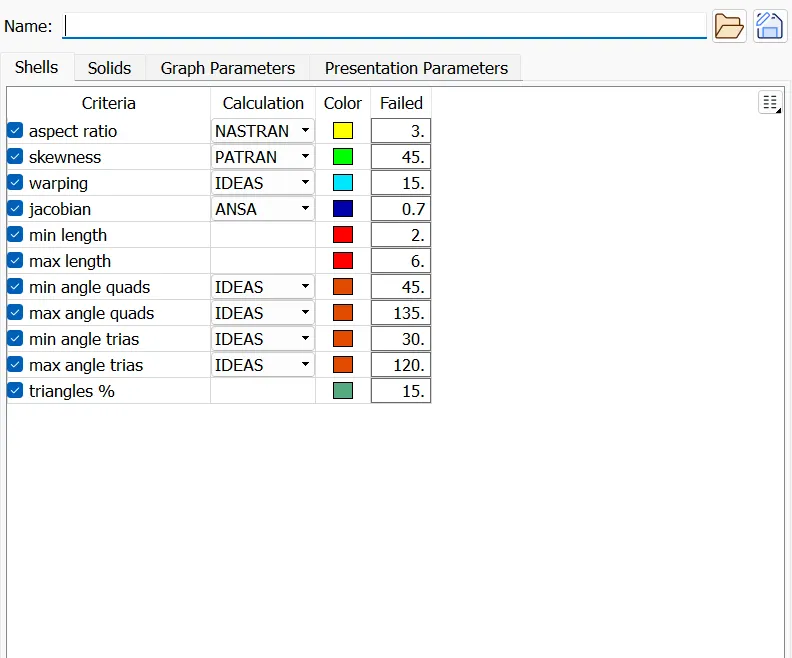
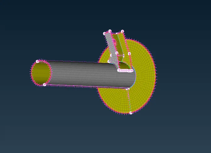
If any failed elements are present we have cleared those elements by using tool split, smooth, reconstruct, paste etc.

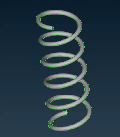
Meshing the spring component.

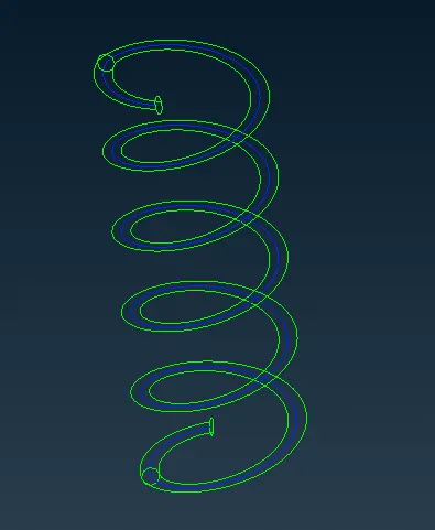
1. For this, we shall be using 1D CBAR elements to represent the part. Firstly, we can generate a middle curve that runs through the entire spring by using the middle tool from the curve options Curves > Middle of the topo deck. We will need to select the cons that run through the entire length of the spring that are on opposite sides of the part as shown:

 

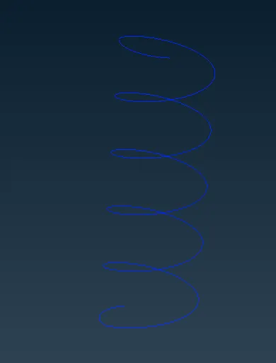
2. After creation of the curve we have to join curve to one curve by using Curves > connect > multi.

3 . The creation of COG point on the curve is done by using the command points > on cog.

4. Having done that, we can move to the NASTRAN deck and go to Elements > CBAR and in the window that pops up, 'orientation with nodes' needs to be checked and the selection needs to be 'Curve (box)'. The curve is then selected and we can click the middle mouse button.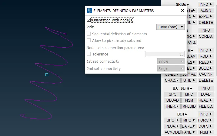

5. After that, we are asked to pick the orientation point and we can select the COG for that. On proceeding, we are to specify the element length as well. We can go for 4mm.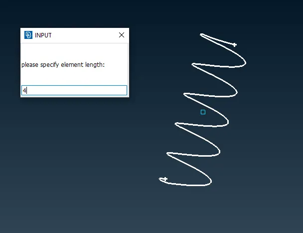

6. After that, on clicking the middle mouse button, we are to assign a property to this curve. We can go ahead and create a new PID. In the next window, we are to input the area (A). In that selection box, we can press Shift + ? to open another window where we simply need to specify the cross-sectional radius of the spring. On doing so, the algorithm automatically calcualtes and populates the other values on the PID card as per the given radius.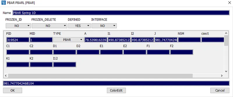

7. In the next window, we need to define the CBAR element by simply naming it. I named it 'spring'.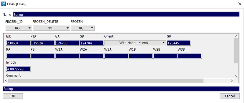



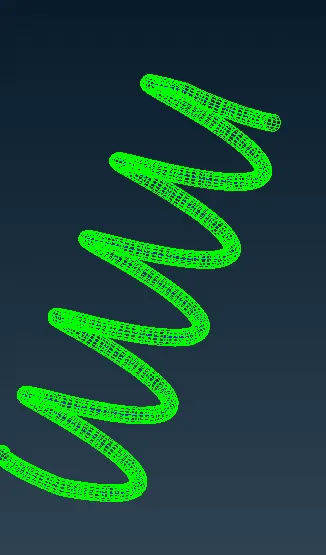
8. On proceeding, we will notice that the 1D elements have been created.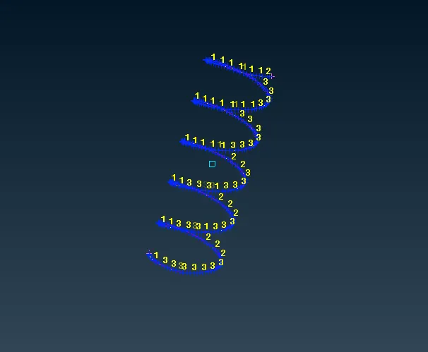

9. These can be represented as 3D solids as well. To do that, we simply need to check the 'Lines Element Cross Section' box and select 'as solids'. These options are available in the presentation parameters tab of the Quality Criteria window.

Connections:

1. All the parts has meshed. we can go through deploying the connections wherever required.

2. To connect regions where a bolt and nut is required, we can use the Two node RBE2 option. The RBE2 tool can be accessed via Elements > RBE2 in the NASTRAN deck. It primarily has the 'many nodes' and 'two nodes' options. This procedure involves connecting two sets of RBE2 spiders using a double con. Firstly, the RBE2 component is created separately for each hole using the Elements > RBE2 > Many Nodes option. We can select the nodes surrounding the hole and the middle mouse click to form the elements.

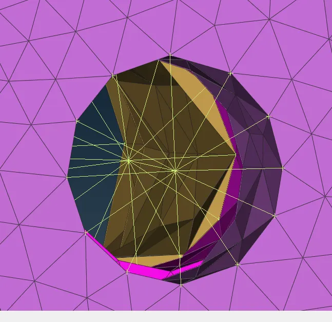
Through this process, we'll have two master nodes (which are to be connected). To connect them, we shall be using the Elements > RBE2 > Two Nodes tool. Then it is just a matter of selecting the two master nodes to form the connection.

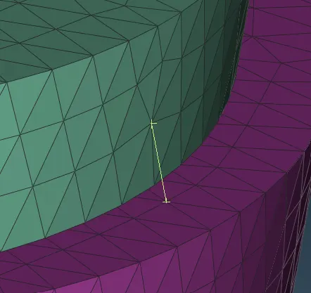
3.The other type of connection we will be deploying in this model is simple two-node RBE2 connections. Not to be confused with the one discussed previously. In this case, we will be providing rudimentary RBE2 connections between two corresponding nodes on different components. This will be used in locations where a shaft-like part/cylindrical part is lowered into a hole. Firstly, we will be selecting Elements > RBE2 > Two Nodes and we will be picking the nodes to be connected as shown:

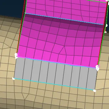
4. Another type of connections are used is seam weld type of connections. For this seam weld we have to create a curve by using the cons2curve.

5. The curve is converted into the seam line by using the command convert > seam line.

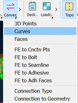
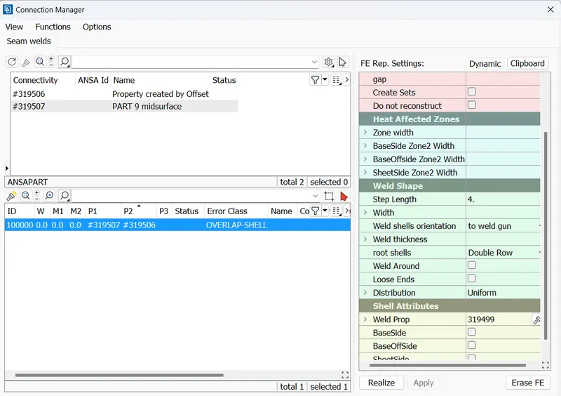
6. Now, we can make use of the connections manager by accessing it from the upper toolbar. The seam line is selected and on proceeding, we get a set of options where we need to tell ANSA what kind of connection we intend on creating. P1 and P2 are selected - To select the PIDs for each, right-click on the option P1 or P2. A box pops up. There, we need to press F1. This will let us select the particular PID. (care must be taken to ensure the right component is selected as the base sheet - the layer on which the weld leg will rest). The FE Rep type here would be Overlap Shell since both layers are parallel to each other.

After that select the double row and apply and realise. The seam weld will be present.

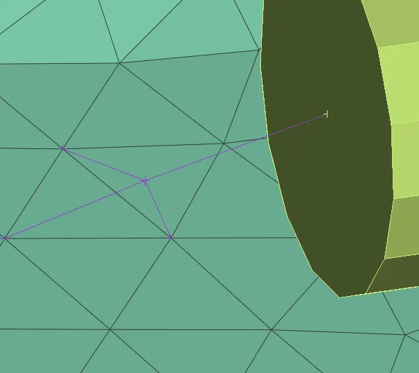
7. finally the connections of the spring to the neighbouring parts as well. For this, we can use cluster RBE2 elements to do so. The process is straightforward. We will need to use the RBE2 tool again. It can be accessed via Elements > RBE2 in the NASTRAN deck. In this case, we deploy the 'many nodes' option to connect the spring and neighbouring part via a single master node. This is also known as a cluster node RBE2.

Reflecting:

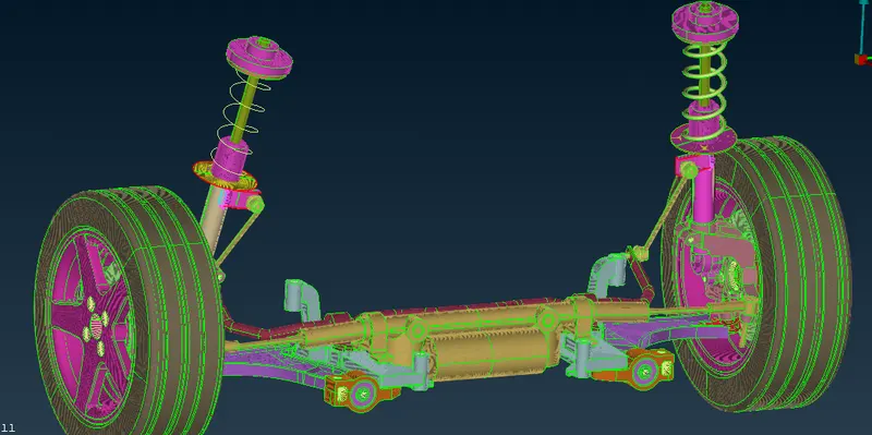
1. After we have meshed the entire model and deployed all possible connections, we can go ahead and reflect it to produce the other half of this rear suspension system. This is done using the reflect option from the Transform tool. 

goto transform > copy. select the entities > select all > middle mouse click > symmetry > mirror 3 point plane > select 3 point. 

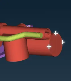
after that apply > middle click > fininsh.

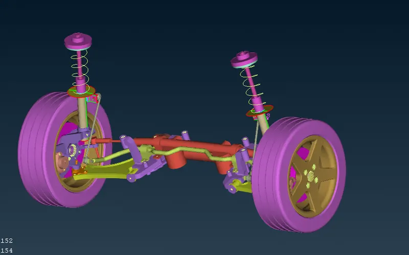
Final models:

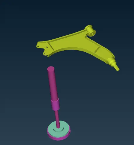
2d meshed models:

 

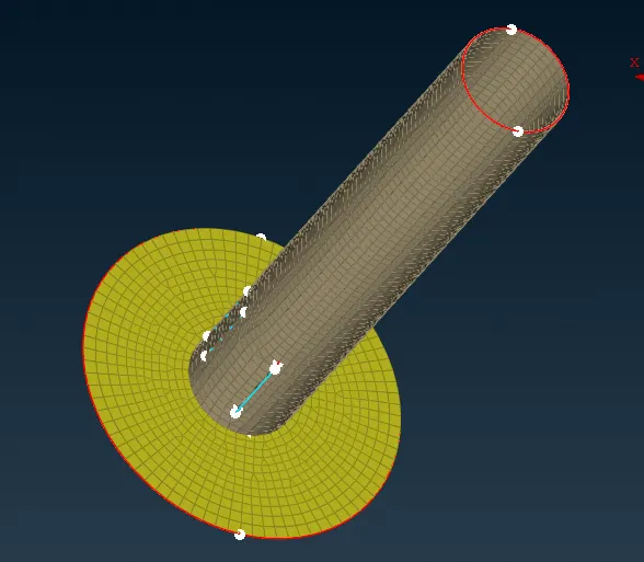
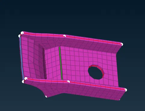
meshed tyre an rim:

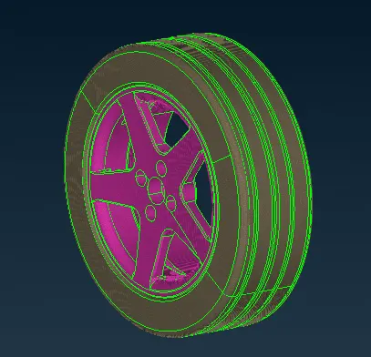
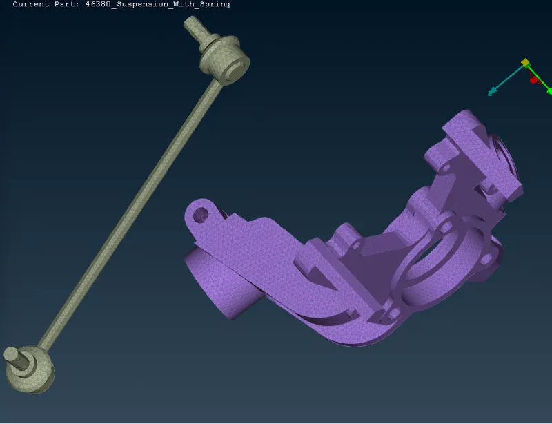
meshed non uniform parts:

 

LEARNING OUTCOMES

1. Through this project, I was able to familiarise myself further with tetra-meshing and connection deployment processes.

2. Learnt to use 1D CBAR elements to represent spring components.

3. Learnt more about various parts involved in a standard suspension assembly.

 RESULT

The given suspension assembly was checked for geometrical errors and fixed accordingly. In addition to that, it was meshed in both 2D and 3D as per the given quality criteria and parameters. Connections were deployed and finally, a symmetrical half was created and reflected to complete the other side of the assembly.