Project - 2 - Meshing on the suspension Assembly
AIM
>> To mesh the given suspension assembly Geometry with both surface and volume mesh with the quality criteria mentioned below.
For Surface Meshing of Tyre and Rim:
|
S.No |
Quality Criteria |
Value |
|
1 |
Target/Average length |
6.5 |
|
2 |
Minimum Length |
5 |
|
3 |
Maximum Length |
10 |
|
4 |
Skewness |
45 |
For Surface Meshing of other Non Uniform thickness components:
|
S.No |
Quality Criteria |
Value |
|
1 |
Target/Average length |
4 |
|
2 |
Minimum Length |
2 |
|
3 |
Maximum Length |
6 |
|
4 |
Skewness |
45 |
For Volume meshing of all Non Uniform thickness components:
|
S.No |
Quality Criteria |
Value |
|
1 |
Tet-collapse |
0.2 |
Quality criteria for Mid surfacing of Uniform thickness part which has thickness less than 5 mm:
|
S.No |
Quality Criteria |
Value |
|
1 |
Target/Average length |
4 |
|
2 |
Minimum Length |
2 |
|
3 |
Maximum Length |
6 |
|
4 |
Aspect |
3 |
|
5 |
Warpage |
15 |
|
6 |
Skewness |
45 |
|
7 |
Jacobian |
0.7 |
|
8 |
Minimum Quad Angle |
45 |
|
9 |
Maximum Quad Angle |
135 |
|
10 |
Minimum Tria Angle |
30 |
|
11 |
Maximum Tria Angle |
120 |
Procedure
>> The given Geometry is imported into ANSA using File>Open.
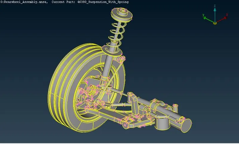
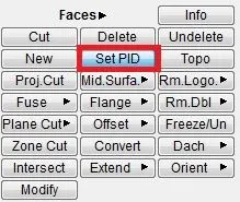
>> The given geometry is sorted on the basis of PID regions, into different PID's for ease of working. This is done using the Faces>Set PID function in the Topo Module.

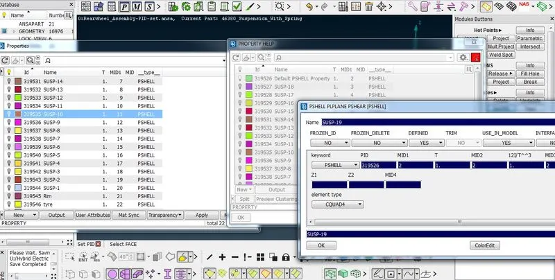
>> Each PID is renamed for easy reference as shown below.
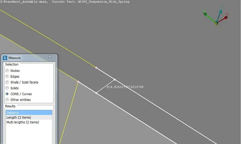
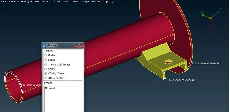
>> Now the thickness of various components are measured using the Utilities>Measure tool and components having thickness below 5 mm are identified.
>> The components identified with thickness less than 5 mm is shown below.
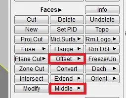
>> The above component is meshed by extracting its midsurface using the offset and middle functions under the Faces section in the Topo Module.
>> The extracted mid surface is shown below.
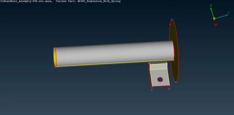
>>After extracting the mid surface, the mid surface is checked for geometric problems using the checks manager
>> Holes are aligned with the nearest edge using Mesh Module>Perimeter>Slide function.
>> To achieve a good quality mesh, holes should be captured by even number of edges. It is done using the 'Module>perimeter>Number' and changed with 'Mesh Module>perimeter>Numb+/-' functions.
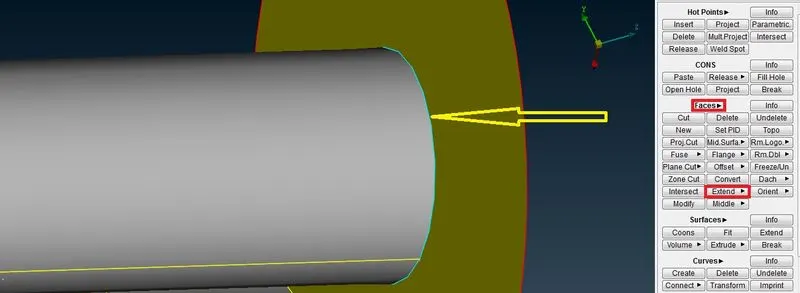
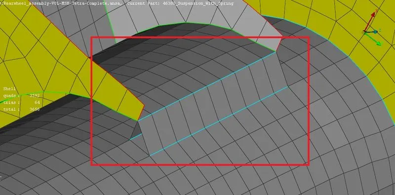
>> The midsurfaces are joined with each other using the extend function under the Faces group in the Topo Module as shown below. Upon joining, the edge colour is changed to cyan indicating that a triple cone is formed there.
>> The component is now meshed as per the required quality parameters by switching to the Mesh module and then selecting 'Spot Mesh' meshing algorithm under 'Mesh generation'. The resulting mesh is again corrected if required by using 'Reconstruct' function under 'shell mesh'. The 'smooth' function is used to obtain smooth mesh lines alignment after obtaining required mesh.
>> During meshing, back to back trias, trias near edges, circular openings and tria concentration are avoided using various tools such as 'Swap', 'Split' and 'Join' functions under 'Elements' in Mesh module. Also the paste function under the 'Grids' is also used to combine adjacent nodes to move the trias away from each other.
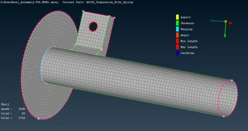
>> The final mesh obtained is shown below.
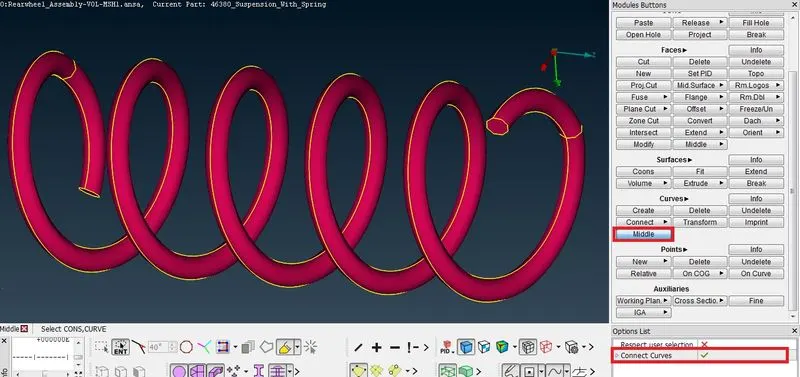
>> To generate the Finite elements for the spring, a middle curve is generated using the middle function under the curves section in the Topo module. The connect curves option is selected to simultaneously join the different curves formed into a single entity.
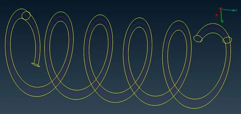
>> After generating the middle curve, a point is formed in the center of gravity of the curve using the 'On COG' function within the Points section in the Topo module.
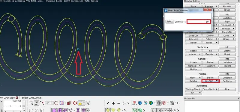
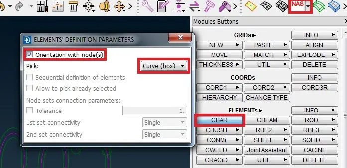
>> Then Solver deck module is selected with NASTRAN solver and under the elements section CBAR is selected. The curve and the point created in the COG is selected.
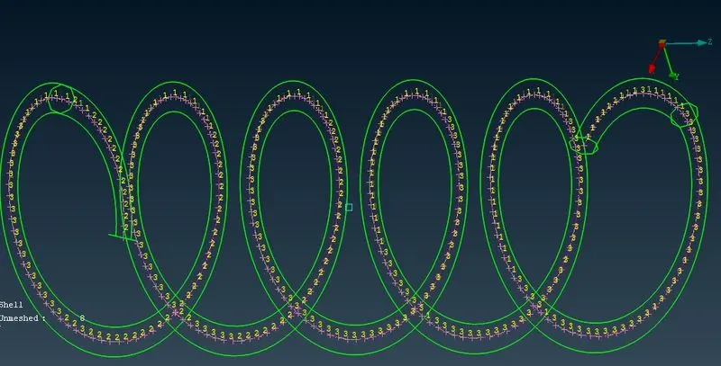
>> The elements generated is shown below.
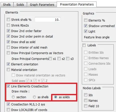
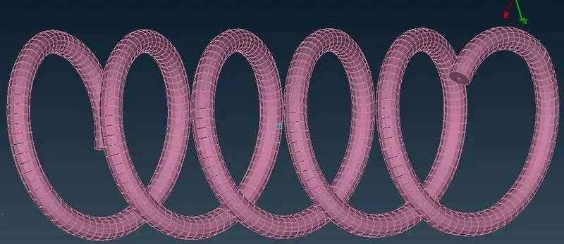
>> Under the presentation parameters, the 'as solids' option is selected for the Line elements CrossSection to visualize the created elements with its thickness as shown below.
>> The remaining components of the geometry are all above 5 mm thickness. Hence they have to be volume meshed as per the criteria given in the question.
>> Before volume meshing the surface is checked for errors and is done by executing the Geometry function under Menubar>Tools>Checks. When execute button is clicked the errors if any are shown and is rectified using the Fix option or by manually checking the area.
>> The orient function under the faces section within Topo module is used to correct the orientation of faces.
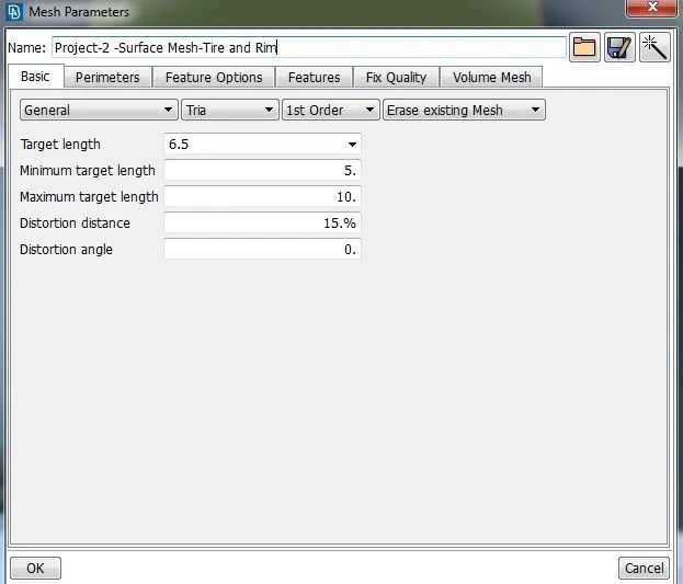
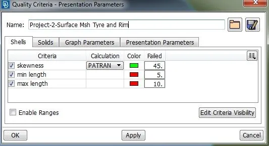
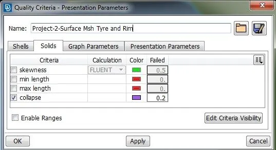
>> For Tire and Rim, the mesh parameters and Quality criteria are entered as shown below. Only collapse value is given for solid volume quality criteria. Also for meshing surface, only Trias are specified.
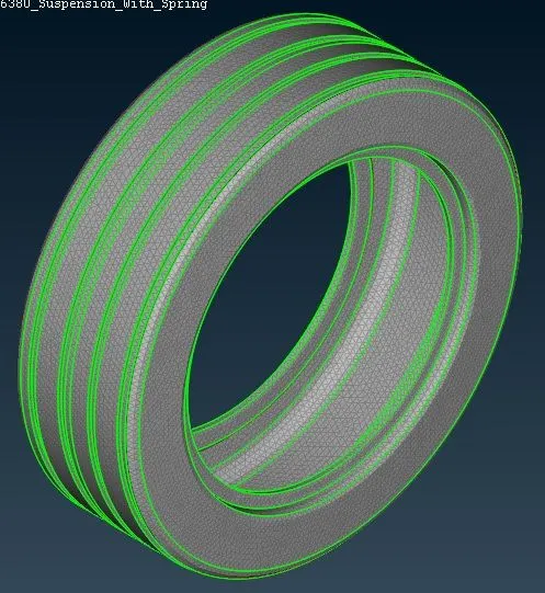
>> The volume mesh generation is same for all the components. The tyre after surface meshing with tria elements is shown below.
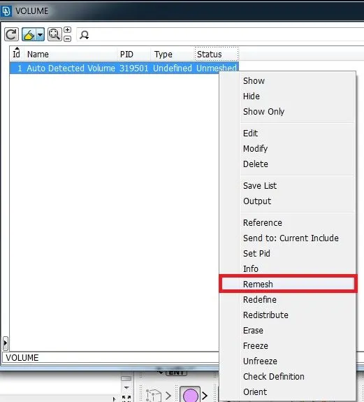
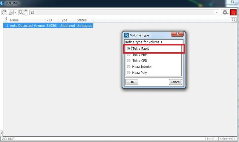
>> The Volume Module is selected. Under the Volumes section, the Define>select function is executed and the tyre is selected. This will create a new volume for volume meshing and can be seen from List function within the Volumes section. The listed volume is right-clicked and Remesh option is given with Tetra Rapid to generate the volume mesh.
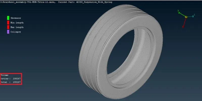
>> The Volume mesh is generated as indicated by the tetras generated as shown below.
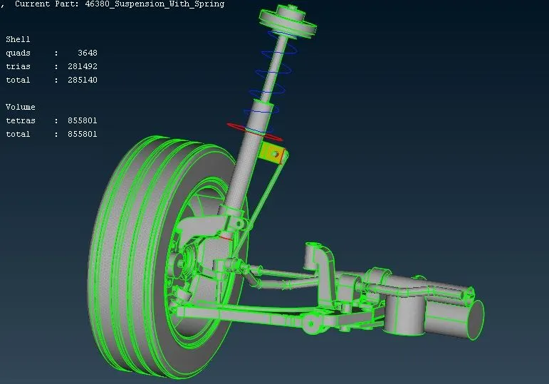
>> This process is repeated for all the remaining components using the specified mesh and quality parameters and the whole geometry mesh is obtained as shown below.
>> To interconnect the components in different PID's together, RBE2 rigid connection and Seam weld is used.
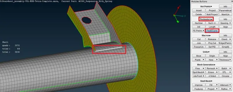
>> To connect with seam weld, the FE element edge is converted into curve using the 'Feat2Curve' function under the Perimeters group in the Mesh module as shown below.
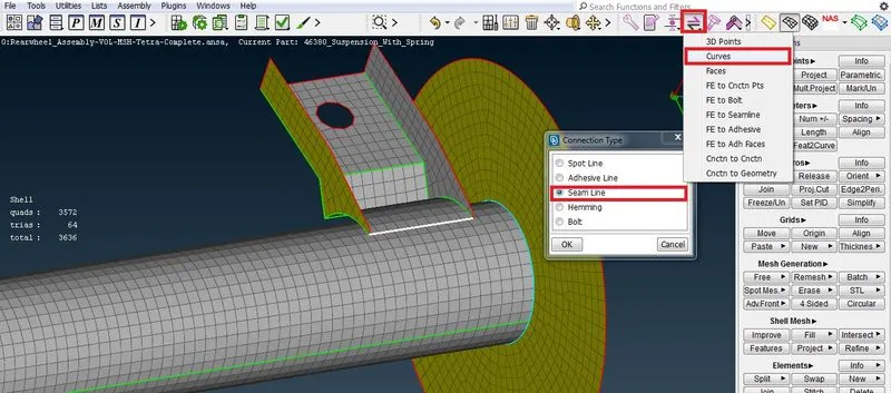
>> This generated curve is conveted into seam line using the convert function in the assembly as shown below.
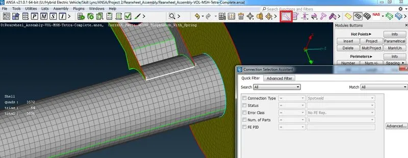
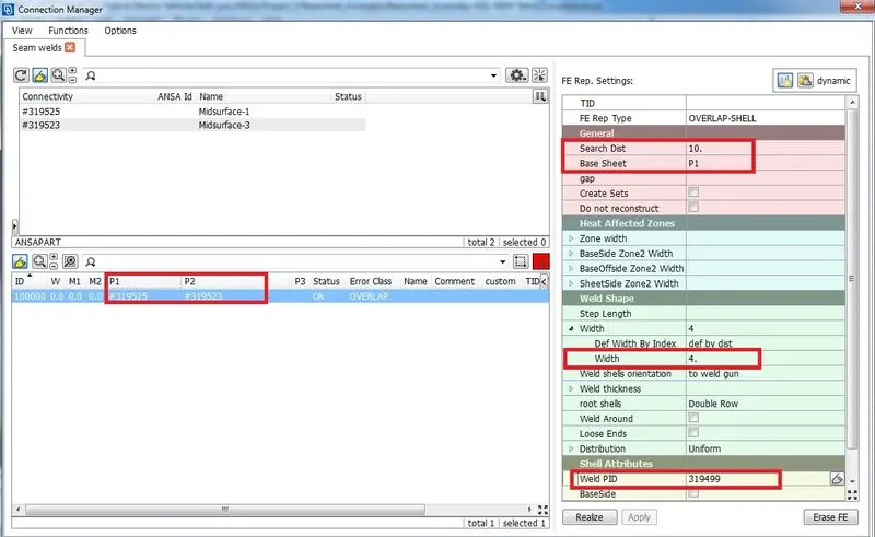
>> Once the seam line is generated, the connection manager is used to create an overlap shell joint with the below shown parameters. P1 and P2 are the PID's of the components to be joined. Thicker one is usually selected as Base sheet. A new weld PID is created for the weld being created.
>> The seam weld created is shown below.
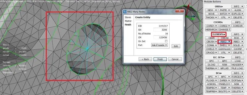
>> Rest of the connections are mostly bolting and is represented by an RBE2 connection rigid connections. This connection is enabled by switching to the Solver module Deck and selecting NASTRAN solver. Then the RBE2 function under the elements area is selected as shown below. The nodes selection loop function is enabled for quicker selection of nodes. Many node RBE2 element is realized as shown below.
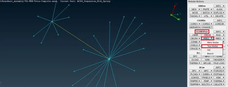
>> To realize a bolt connection, the two node RBE2 is formed between master nodes of the two many noded RBE2 element as shown below.
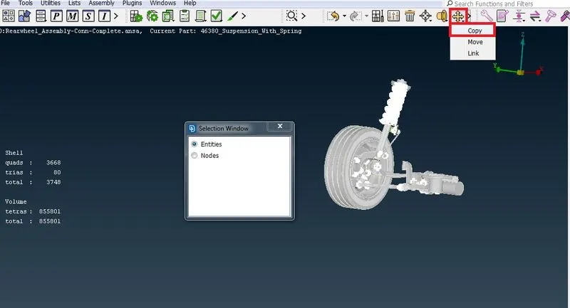
>> Once all the required connections are given, the FE model is reflected to the other side using the Transform>Copy function as shown below.
>> Three nodes are selected in the plane across which the reflection is to be done
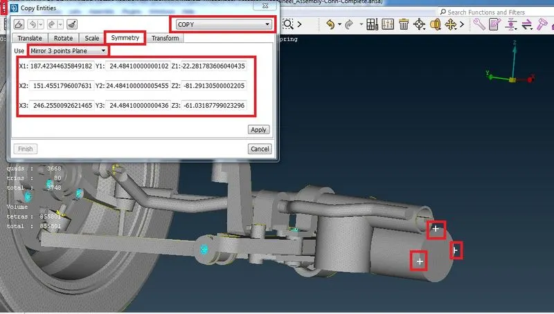
>> The reflected model is shown below.
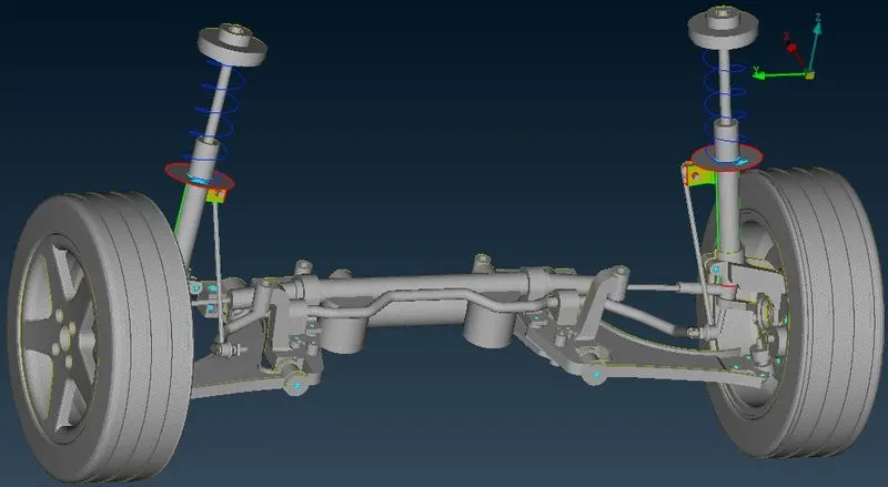
>> 'Draw shell as solids' and 'Line Elements CrossSection' as solids option is enabled for 3-d visualization of the suspension assembly.
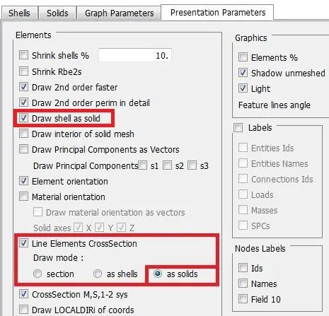
>> The final meshed output of the Suspension assembly along with the required connections is shown below.
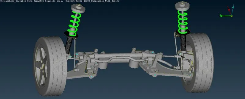
Learning Outcomes
>> Acquired idea of sorting and meshing a model with both sheet metal and non uniform thickness components together.
>> Practiced meshing of sheet metal components and volumetric meshing within the same model.
>> Practised Symmetry command and deployed and realized various type of connections using appropriate FE representative elements such as RBE2 for bolt connections, Seam weld connection.
Conclusion
>> Using systematic approach, the given Suspension assembly was modelled using 2d and 3d elements and interconnected with suitable connections successfully.