Project 2

Project 2 - Development of a forward energy-based fuel consumption model of a P1 hybrid vehicle.

This project consists of modelling of forward energy fuel consumption of a P1 Hybrid vehicle by using MATLAB and SIMULINK. We have seen that in previous Project 1 of Conventional vehicle the Engine was only the power source, but in hybrid vehicle it is not only the Engine that generates power, it has the Motor and Bttery syatem also.

HEV

Hybrid electric vehicles are powered by an internal combustion engine and one or more electric motors, which uses energy stored in batteries. A hybrid electric vehicle cannot be plugged in to charge the battery. Instead, the battery is charged through regenerative braking and by the internal combustion engine. The extra power provided by the electric motor can potentially allow for a smaller engine. The battery can also power auxiliary loads and reduce engine idling when stopped. Together, these features result in better fuel economy without sacrificing performance.

So the model is built by considering Engine, Motor and Battery.

Before building the simulink model various parameters are to be defined to control the performance of the vehicle components. This parameters can be listed in the MATLAB script file mentioned below. The drive cycle can be selected by giving the appropriate numbers from 1 to 6 in the Drive_cycle_select command.

List of parameters

%%%%%%%%%%%%%%%%%%%%%%%%%%%%%%%%%%%%%%%%%%%%%%%%%%%%%%%%%%%%%%%%%%%%%
%% Skill-Lync -> Hybrid Drives Development
% Project 2 - Development of a forward energy-based fuel consumption model of a P1 hybrid vehicle.

% By - Deep Makwana

% Description: This script file contains the necessary or input values to be considered while modeling the P1 Hybrid vehicle. The below contents represents the vehicle parameters, Powertrain parameters and the vehicle
% data taken from ADVISOR data base developedby NREL, USA. This vehicle data is loaded from the specified folder. The script also contains the selection of desired drive cycle from the folder.

%% Initialization File
% Initialization file for loading the variables for the Conventional vehicle simulation model

%% Vehicle Parameters

M = 1500; % Vehicle weight [kg]
Cr = 0.015; % Rolling resistance coefficient
Rw = 0.35; % Rolling radius [m]
Cd = 0.33; % Drag coefficient
Af = 2; % Frontal area [m2]
rhoa = 1.225; % Air density [kg/m3]
Vwind = 0; % Wind velocity [kmph]
g = 9.81; % Gravitational acceleration [m/s2]
theta = 0; % Slope [deg]
myu_road_tire = 1; % Coefficient of friction between tire - road interface

%% Powertrain Parameters

FDR = 3.73; % Final Drive Ratio / Diff Ratio
DiffEff = 0.99; % Differential efficiency (assumed independent of operating conditions)

NumGear = 4; % Number of gears in transmission
TransGear = [1:NumGear]; % Transmission Gears
TransRatio = [3.06, 1.62, 1, 0.7]; % Corresponding Transmission ratios
TransEff = 0.90; % Transmission efficiency (assumed independent of operating conditions)

TC_SR = [0, .5, .6, .7, .8, .87, .92, .94, .96, .97, 1]; % Torque Converter Speed Ratio (Matlab default) -> TurbSpd/PumpSpd
TC_TR = [2.232, 1.5462, 1.4058, 1.2746, 1.1528, 1.0732, 1.0192, 1, 1, 1, 1]; % Torque Converter Torque Ratio (Matlab default) -> TurbTrq/PumpTrq
TC_Cf = 1e-4 * [.72558, .66322, .63463, .59042, .51331, .4144, .29287, .22444, .12186, .04386, 0]; % Torque Converter Capacity Factor (Matlab default) -> PumpTrq/PumpSpd^2 [Nm/rpm^2]

load Vehicle_Data/Engine_data_1_9L_Saturn_95kW
load Vehicle_Data/Trans_Shift_map
load Vehicle_Data/EM_Honda_Insight_10kW
load Vehicle_Data/ESS_NiMH6

ESS_init_soc = 0.8;
ESS_soc_max = 0.9;
ESS_soc_min = 0.6;

%% Driver Parameters
Kp = 10; % P gain for driver PI model
Ki = 1; % I gain for driver PI model
Drive_Cycle_Select = 1; % Drive cycle selection

% Drive cycle values in m/s

if Drive_Cycle_Select == 1
load DriveCycles/UDDS;

elseif Drive_Cycle_Select == 2
load DriveCycles/HWFET;

elseif Drive_Cycle_Select == 3
load DriveCycles/FTP;

elseif Drive_Cycle_Select == 4
load DriveCycles/US06;

elseif Drive_Cycle_Select == 5
load DriveCycles/NEDC;

elseif Drive_Cycle_Select == 6
load DriveCycles/WLTP;

end

time_end = cyc_time(end);
vel_end = cyc_vel(end);

After defining the parameters and running the script now the SIMULINK model is built by considering the architecture of P1 hybrid as below.

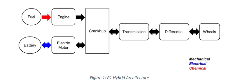
The SIMULINK model for hybrid vehicle is very much similar to the conventional model apart from considering certain changes in parameters due to addition of the Electric Motor and Battery units. And as asked, the model will be running on two drive cycles namely, UDDS and HWFET.

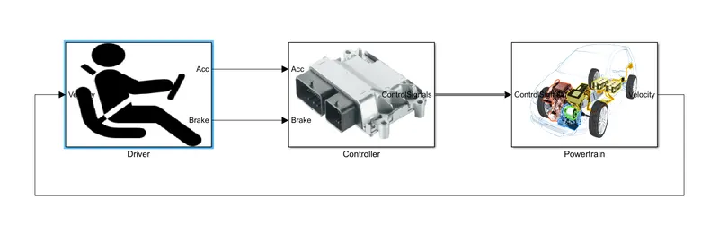
Similar to conventional, the hybrid model also consists of 3 primary systems known as, The Driver, Controller and Powertrain containing various subsystems as shown below.

1) Driver model

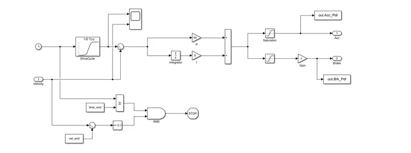
The Driver model for the P1 Hybrid will be same as the conventional model in Project 1. There are no changes in it.

2) Controller model

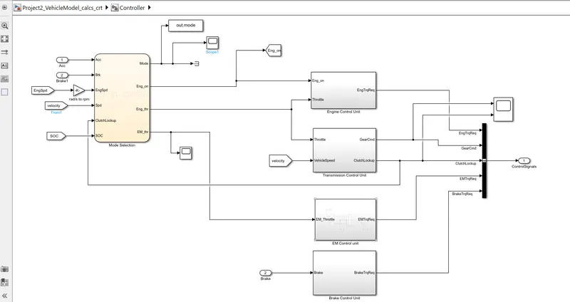
There is addition of Mode Selection block and an Electric Motor Control Unit block in the controller model as shown below.

• Mode Selection unit

The Mode selection block is a Stateflow Chart block which contains various inputs and outputs. Inside Mode selection, 4 states representing the different operating modes of the vehicle are connected to each other as shown below.

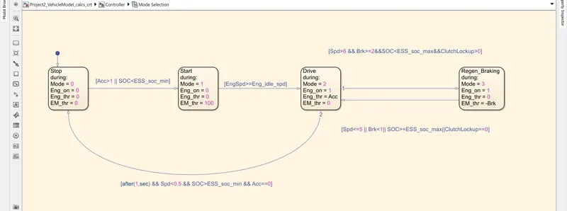
The 4 states represents state of the vehicle as;

i) Stop - It is the state when the vehicle is at stop condition. Both the Engine and Motor is at off condition.

ii) Start - It is the state when the vehicle is started is about to move. At this stage the vehicle gets its initial throttle power from the Motor and the Engine is still off.

iii) Driving - In this state the vehicle starts running and is power by the Engine at high speeds and more power requirement.

iv) Regenerative Braking - At this stage the brakes are applied to the vehicle and is retarding to low speeds. Power generated at the wheels due to braking is used to charge the battery system.

The transfer from one state to the other depends on the conditions mentioned between the states.

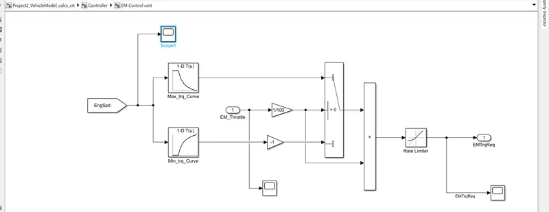
• EM Control unit

Electric Motor control unit supplies or control power from the battery depending on the speed of the vehicle. EM control unit identifies the amount of power and torque required and runs the electric motor at desired conditions.

• Engine control unit

The Engine control unit of the Hybrid model takes one extra input of "Eng_on" as compared to conventional vehicle model. This is then feed to idle speed controller which determines the Engine on & off conditions and regulates the speed input values. The rest of the things are common to the conventional vehicle model.

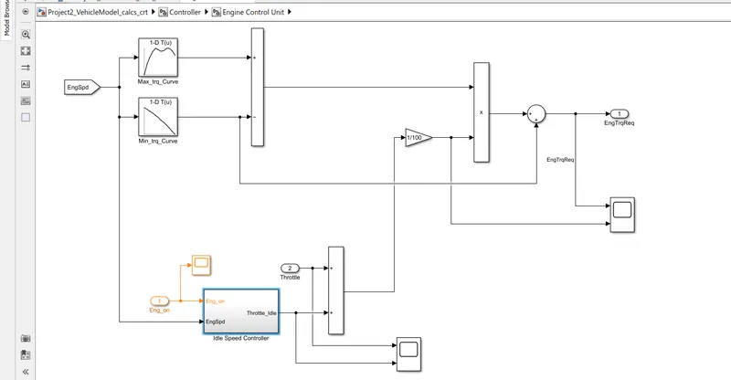
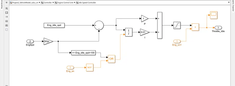
We can see that the engine control unit has an idel speed controller which makes sure that the engine is idling and does not go below the idle speed. The idle speed controller is again a PI controller having different gain values. This idle speed controller is then added to throttle which then converted to engine torque based in the max and min curve values.

• Transmission Control Unit

The Transmission unit takes in the Throttle and Velocity as input and gives Gear command as output. It has an additional output called "ClutchLockup". It is the torque converter clutch in between the pump and turbine giving the torque converter values while engaging and disengaging. If the ClutchLockup value is 1 then we need to lock up the clutch and if the ClutchLockup is 0 it means clutch is open.

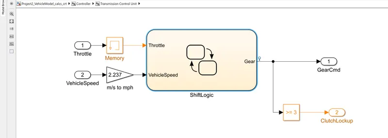
As shown above it consists the same shiftlogic block as in conventional vehicle. Only the change is, if the gear is above or equal to 3rd gear we want to lockup the clutch and if it is less than 3rd gear it will be open.

• Brake Control Unit

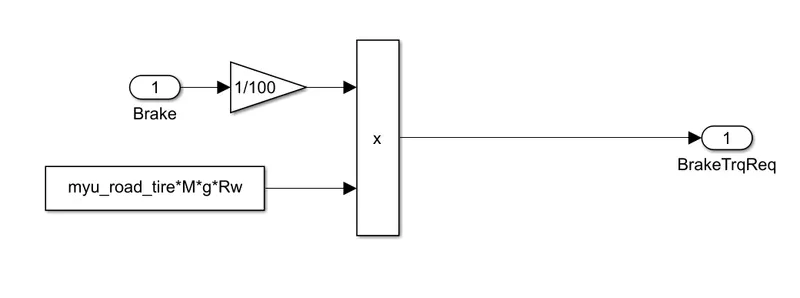
The Brake control unit also remains same as in conventional vehicle model, there are no changes.

3) Powertrain model

Powertrain is the source of power generation in the vehicle. It is the most important unit of vehicle which regulates the performance of the vehicle. A good quality powertrain is a key to a better operating range, acceleration, and top speed. So, when you accelerate your car from a standstill and feel a push of your engine power, just know that your powertrain propelled your vehicle.

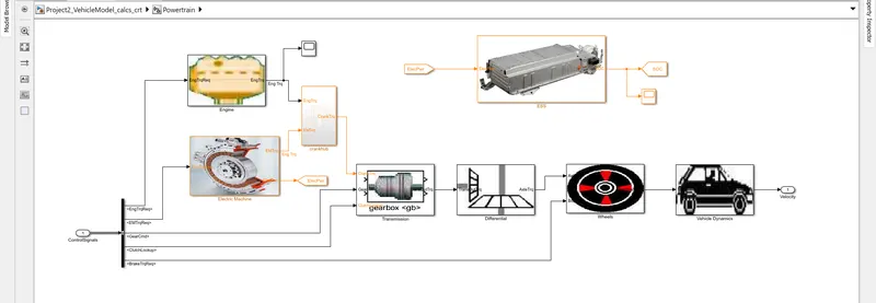
The simulink model for the powertrain is shown in the below picture. As in hybrid vehicle the power source is Engine and Battery both so the model consists extra units as Electric Machine (motor) and Energy storage system (Battery) as mentioned below. It also consists of Crankhub which is used to add both engine torque and motor torque giving the total torque output.

• Engine Unit

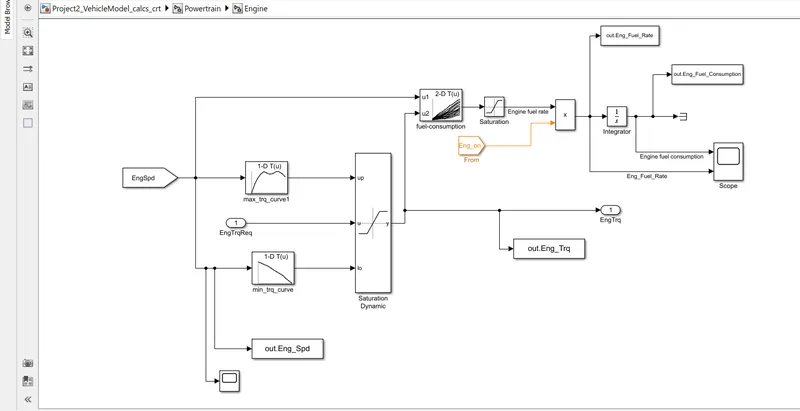
The change in the engine unit is that we multiply an "Engine on" function block to the engine fuel rate output. The rest of the parameters and input output blocks are same to the conventional model.

• Electric motor

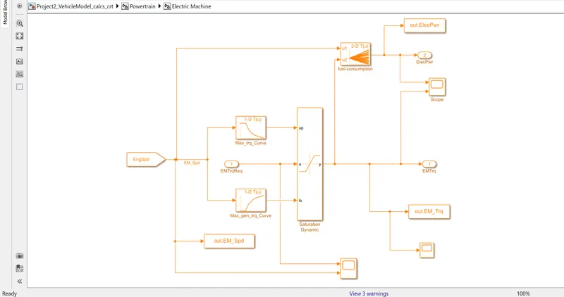
The inputs to the electric motor are torque and engine speed. This speed input goes to the maps to generate max torque curve and min torque curve. This torque values are generated to saturate the required torque value. The motor torque is comming from the EM control unit. The saturated toeque values along with engine speed values is then feed to fuel consumption map giving the electrical power as output. The setup for this model can be seen in the below picture.

• Crankhub

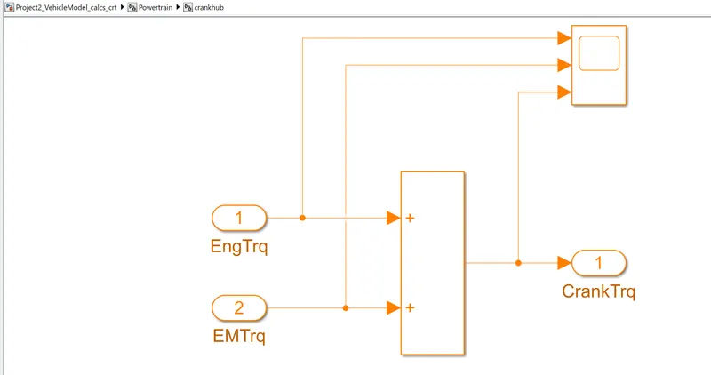
Crankhub is just simple block to add the Engine torque and Electric Motor torque resulting in the Total torque or Crank torque as output.

• Energy Storage System (Battery)

The ESS takes input as electric power from the electric motor. This power is used to run the accessories and also to run the vehicle at low speeds or meets the initial starting power requirements. Output from the battery is the State of Charge (SOC) which goes and feed back to the Mode Selection or Supervisory Controller. The SOC represents the state of battery like, the amount of power in the battery. The construction of ESS system can be seen below.

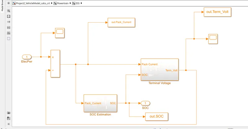
We can see from the above figure that ESS also contains two sub blocks called SOC Estimaton and Terminal Voltage blocks which can be discussed as folows;

i) SOC Estimation

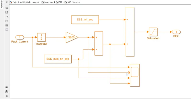
This block takes in current from the pack current and based on the current capacity it gives the state of charge values. The SOC value is obtaind by subtracting Used SOC from the Initial SOC as shown in the below figure.

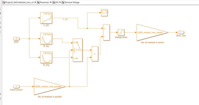
ii) Terminal Voltage block

Terminal voltage block takes in the Pack Curent and then checks the number of modules connected in parallel. It also takes SOC as input and feed this values to Open Circuit voltage (V_OC), and Internal Resistance creating the map values of the modules connected in series. The internal resistance values are divided as Internal Resistence Discharge and Internal Resistance Charge which are connrctrd to switch block. The switch block chooses the resistance value base on charging and discharging conditons. This resistance value and the pack current value is multiplied together and then subtracted from the open circuit voltage resulting in Terminal Voltage value.

• Transmission unit

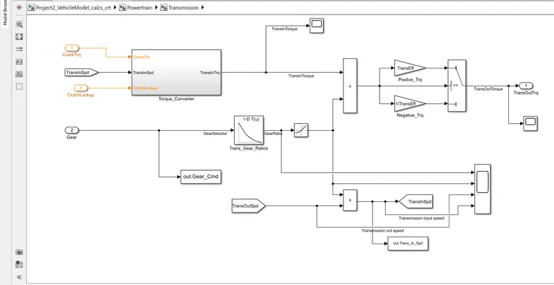
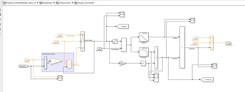
In hybrid model the Transmission has 3 inputes instead of 2 as in conventional model. The transmission takes Crank torque as input and this crank torque values goes to torque converter based on which the Engine dynamics are defined. The Engine Dynamics now has both Engine inertia and Motor inertia added together which is then provided to the switch block.

The torque converter block also has two more inputs as Trans in speed and Clutchlockup which is also feed to switch block. This switch block identifies the clutch open or close condition and based on that gives turbine speed or pump speed as output.

• The Differential, Wheels and Vehicle Dynamics model are same as conventional model in Project 1.

Now after building and running the simulink model various plots are made to observe the performance of each components of the hybrid vehicle. Below is the MATLAB script file which contains the plotting commands and the result values obtained.

Post-Processing script file

%%%%%%%%%%%%%%%%%%%%%%%%%%%%%%%%%%%%%%%%%%%%%%%%%%%%%%%%%%%%%%%%%%%%%%% Skill-Lync -> Hybrid Drives Development
% Project 2 - P1 Hybrid Vehicle Model

% By - Deep Makwana

% Description: A MATLAB script is Created to analyse data and to generate plots. Here we rename the variables loaded from the model, do some basic post-process calculations and generate results and plots.
The following file is to used with the Initialization file and Simulink results for post-processing of the data. The file is incomplete, has some examples of how the data is imported into a readable format, data analysis and plotting examples. Based on the project task, use commands in a similar format as given below, to analyse the data and generate required plots. Variable names can be changed if desired.

%% Post-Processing File
% File for post-processing the Conventional vehicle simulation model data

%% Renaming variables

Time = out.tout;
Acc_Pdl = out.Acc_Pdl; % Accelerator pedal [%]
Brk_Pdl = out.Brk_Pdl; % Brake pedal [%]
Gear_Cmd = out.Gear_Cmd; % Transmission gear
Trans_In_Spd = out.Trans_In_Spd*30/pi; % Transmission input speed [rpm]
Trans_Out_Spd = out.Trans_Out_Spd*30/pi; % Transmission output speed [rpm]
Eng_Trq = out.Eng_Trq; % Engine brake torque [Nm]
Eng_Spd = out.Eng_Spd*30/pi; % Engine speed [rpm]
Eng_Fuel_Consump = out.Eng_Fuel_Consumption; % Engine fuel consumption [g]
Eng_fuel_rate = out.Eng_Fuel_Rate; % Engine furl rate in (g)
Veh_Dist = out.Veh_Dist/1000; % Distance traveled by vehicle [km]
veh_des_spd = out.veh_des_spd*18/5; % Vehicle desired speed
Veh_Spd = out.Veh_Spd*18/5; % Vehicle speed [kmph]
Wheel_Speed = out.WheelSpeed; % Wheel speed [kmph]
Eng_Fuel_Rate = out.Eng_Fuel_Rate; % Engine fuel rate [%]
EM_Speed = out.EM_Spd*18/5; % Electric Motor Speed
EM_Power = out.ElecPwr; % Electric Motor Power
EM_Torque = out.EM_Trq; % Electric Motor Torque
Term_Volt = out.Term_Volt; % Terminal Voltage of battery
Soc = out.SOC; % State Of Charge
Pack_Current = out.Pack_Current; %Pack current of battery

%% Data Analysis

Eng_Pwr = (Eng_Spd*pi/30).*(Eng_Trq/1000); % Engine brake power [kW]
rho_petrol = 0.7197; % Density of petrol [kg/L]
kmpl = Veh_Dist(end)/(Eng_Fuel_Consump(end)/1000/rho_petrol); % Fuel economy [kmpl]

%Eng_spd = Eng_Spd.Data(:,1); % engine speed
%Eng_trq = Eng_Trq.Data(:,1); % engine torque
%Eng_pwr = Eng_Pwr.Data(:,1); % engine power
%Eng_fuel_rate = Eng_Fuel_Rate.Data(:,1); % engine fuel rate
%Eng_fuel_consumption = Eng_Fuel_Consump.Data(:,1); % engine fuel consumption
%EM_speed = EM_Speed.Data(:,1); % motor speed
%EM_power = EM_Power.Data(:,1); % Motor Power
%EM_torque = EM_Torque.Data(:,1); % Motor Torque
%Pack_current = Pack_Current.Data(:,1); %pack current of battery
%State_of_charge = Soc.Data(:,1); %state of charge
%Term_voltage = Term_Volt.Data(:,1); % terminal Voltage of battery

%% (b) Plotting of time trace for engine, transmission input, transmission output and wheel speed
figure('Name','(plot b) Engine torque, Trans. in, Trans. out, wheel speed');
hold on
grid on
plot(Time, Eng_Spd,'r','linewidth',1);
plot(Time, Trans_In_Spd,'b','linewidth',1);
plot(Time, Trans_Out_Spd,'y','linewidth',1);
plot(Time, Veh_Spd,'g','linewidth',1);
xlabel('Time (s)')
ylabel('speed (rpm)')
legend('Engine speed','Trans input spd','Trans output spd','Wheel speed');

%% (c) Plotting engine torque, engine power, fuel rate, fuel comnsumption.
figure('Name','(plot c) Engine torque,power,fuel rate, fuel conp.');
subplot(4,1,1)
hold on
grid on
plot(Time, Eng_Trq,'b','linewidth',1); xlabel('Time'); ylabel('Torque')
subplot(4,1,2)
hold on
grid on
plot(Time, Eng_Pwr,'r','linewidth',1); xlabel('Time'); ylabel('Power')
subplot(4,1,3)
hold on
grid on
plot(Time, Eng_Fuel_Consump,'k','linewidth',1); xlabel('Time'); ylabel('Fuel consumption')
subplot(4,1,4)
hold on
grid on
plot(Time, Eng_fuel_rate,'g','linewidth',1); xlabel('Time'); ylabel('fuel rate')

%% (d) Plotting vehicle characteristics time trace
figure('Name','(plot d) vehicle characteristics time trace')
subplot(4,1,1)
hold on
grid on
plot(Time, Acc_Pdl, 'linewidth', 1, 'Color', 'black');
plot(Time, Brk_Pdl, 'linewidth', 1, 'Color', 'red');
ylabel('Pedal [%]')
xlim([0, Time(end)]);
legend('Accel','Brake');
subplot(4,1,2)
hold on
grid on
plot(Time, veh_des_spd, 'linewidth', 1, 'Color', 'black');
plot(Time, Veh_Spd, 'linewidth', 1, 'Color', 'red');
ylabel('Speed [rpm]')

legend('Vehicle desired speed','Vehicle actual speed');
subplot(4,1,3)
hold on
grid on
plot(Time, Gear_Cmd, 'linewidth', 1, 'Color', 'black');
xlim([0, Time(end)]);
xlabel('Time [s]');
ylabel('Gear');
subplot(4,1,4)
hold on
grid on
plot(Time,Veh_Dist,'y','linewidth',1); xlabel('Time'); ylabel('vehicle distance (km)')

%% (e) Plotting engine operating points on engine fuel map
figure('Name','(plot e) Engine Operating Points');
hold on
grid on
title('Engine Operating Points','fontsize',12);
p1=plot(Eng_map_spd*30/pi,Eng_max_trq,'linewidth',2,'color','r');
p2=line([Eng_map_spd(end)*30/pi Eng_map_spd(end)*30/pi],[0 Eng_max_trq(end)]);
set(p2,'linewidth',1,'linestyle','--','color','k');
p3=line([Eng_map_spd(1)*30/pi Eng_map_spd(1)*30/pi],[0 Eng_max_trq(1)]);
set(p3,'linewidth',1,'linestyle','--','color','k');
[c,h] = contour(Eng_map_spd'*30/pi,Eng_map_trq,Eng_fuel_map');
clabel(c,h);
xlabel('Engine Speed [rpm]');
ylabel('Engine Torque [Nm]');
title('Engine Fuel Consumption Map [g/s]');
p4 = plot(Eng_Spd,Eng_Trq,'.','color','k');
legend([p1 p4],{'Max Curve','Operating Points'});
axis([Eng_map_spd(1)*30/pi Eng_map_spd(end)*30/pi 0 Eng_map_trq(end)]);

%% (f) Plotting of motor speed, torque, motor input power
figure('Name','(plot f) motor speed, torque, motor input power');
subplot(3,1,1)
hold on
grid on
plot(Time, EM_Speed,'r','linewidth',1); xlabel('Time'); ylabel('Motor speed')
subplot(3,1,2)
hold on
grid on
plot(Time,EM_Torque,'b','linewidth',1); xlabel('Time'); ylabel('Motor torque')
subplot(3,1,3)
hold on
grid on
plot(Time,EM_Power,'g','linewidth',1); xlabel('Time'); ylabel('Moter power')

%% (g) Plotting of Pack voltage, current and SoC
figure('Name','(plot g) Pack Voltage, Pack Current, SoC');
subplot(3,1,1)
hold on
grid on
plot(Time,Term_Volt,'r','linewidth',1); xlabel('Time'); ylabel('Terminal Voltage')
subplot(3,1,2)
hold on
grid on
plot(Time,Pack_Current,'g','linewidth',1); xlabel('Time'); ylabel('Pack Current')
subplot(3,1,3)
hold on
grid on
plot(Time,Soc,'g','linewidth',1); xlabel'('Time'); ylabel('SOC')

%% (h) Plotting of motor operating points on the motor input power map

figure('Name','(plot h) Motor Operating Points');
hold on
grid on
title('Motor Operating Points','fontsize',12);
p1=plot(EM_map_spd*30/pi,EM_max_trq,'linewidth',2,'color','r');
p2=line([EM_map_spd(end)*30/pi EM_map_spd(end)*30/pi],[0 EM_max_trq(end)]);
set(p2,'linewidth',1,'linestyle','--','color','k');
p3=line([EM_map_spd(1)*30/pi EM_map_spd(1)*30/pi],[0 EM_max_trq(1)]);
set(p3,'linewidth',1,'linestyle','--','color','k');
[c,h] = contour(EM_map_spd'*30/pi,EM_map_trq,EM_inpwr_map');
clabel(c,h);
xlabel('Motor Speed [rpm]');
ylabel('Motor Torque [Nm]');
title('Motor Fuel Consumption Map [g/s]');
p4 = plot(EM_Speed,EM_Torque,'.','color','k');
legend([p1 p4],{'Max Curve','Operating Points'});
axis([EM_map_spd(1)*30/pi EM_map_spd(end)*30/pi 0 EM_map_trq(end)]);

Tasks:

(a) Fuel economy numbers (kmpl)

	UDDS	HWFET
kmpl	20.44	33.74

As UDDS cycle belongs to the city driving conditions the fuel economy of this cycle will be less than HWFET cycle. The reasons behind less economy is the uneven road conditions resulting in frequent braking and accelerating the vehicle, more traffic and signal conditions in city resulting in idling of vehicle etc. Whereas the HWFET belonging to highway driving conditions has better road conditions, very less traffic and no signals resulting in more fuel economy.

Plotting of parameters

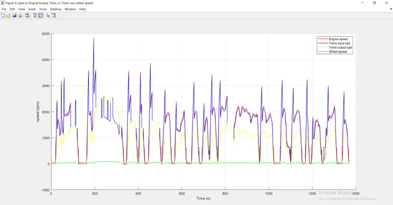
• (b) Plots of time trace for engine, transmission input, transmission output and wheel speed

UDDS cycle

HWFET

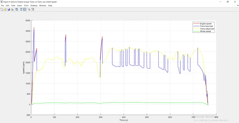
The above plot represents the Engine, Transmission and Wheel speed curves with respect to time in single figure. In the above plot red lines indicate Engine speed, blue lines indicate Transmission input speed, yellow line indicates Transmission output speed, and green line indicates the Wheel speed. We can see that as the engine components are rotating at very high rpm or speed as compared to the vehicle velocity, so the plot values for this engine and transmiddion components are high as compared to wheel speed values.

The Engine and Transmission values are fluctuating more due to the city driving condition in UDDS cycle as compared to HWFET cycle.

• (c) Plots of engine torque, engine power, fuel rate, fuel comnsumption.

UDDS

HWFET

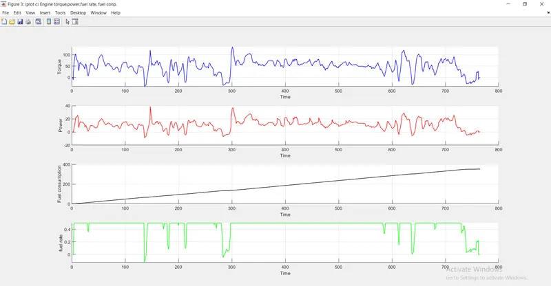
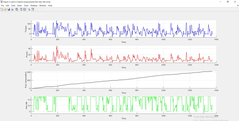
The above figures contains 4 plots representing Torque, Power, Fuel consumption and Fuel rate against Time. From the above plot of fuel rate and power we can see that the fuel consumption is more for high power requirement of the vehicle. But as the UDDS cycle belongs to city driving conditions, the power requirement is less as compared to highway driving in HWFET cycle. So the total fuel consumption is less in the UDDS cycle as compared to HWFET.

• (d) Plot of vehicle characteristics time trace.

UDDS

HWFET

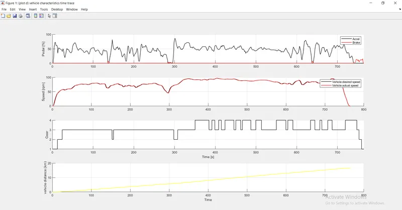
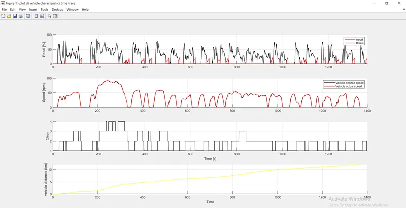
The above figure also has 4 plots representing the Acceleration & Brake pedal, vehicle Desired & Actual speeds, Gear command, and Vehicle distance curves with respect to Time. As the UDDS cycle belongs to city driving conditions which has more traffic, signals, uneven road conditions etc resulting in the frequent decrease and increase in the speed of vehicle which leads in pressing the brake pedal various times in the driving. So we can see that the UDDS cycle has more brake curves as compared to HWFET cycle.

Due to more variations in speeds the shifting of Gears in UDDS cycle is also more as compared to HWFET which can be seen in the 3rd subplot in the both figures.

• (e) Plot of engine operating points on engine fuel map

UDDS

HWFET

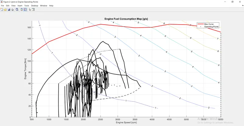
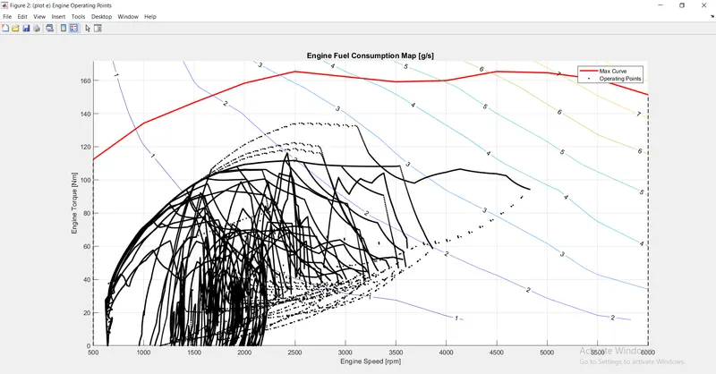
This figures contain plot of engine operating points like Engine speed and torque considering the fuel consumption parameter. In the figure Red line indicates the max torque curve at the perticular speed. The Black dots represents operating points at speed and torque values. The color lines indicates the fuel consumption at perticular speed and torque.

• (f) Plot of motor speed, torque, motor input power

UDDS

HWFET

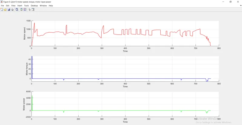
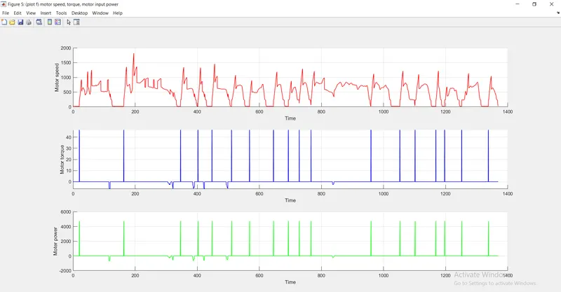
The above figure contains 3 plots namely Motor speed, Motor torque, Motor power with respect to time. In city driving conditions the power and speed of vehicle keep on varing which results in the working of motor again and again at low speeds or at initial starting conditions. But as the HWFET cycle is the highway cycle and the vehicle can run at a constant speed, and the power and torque at high speeds is provided by the Engine.

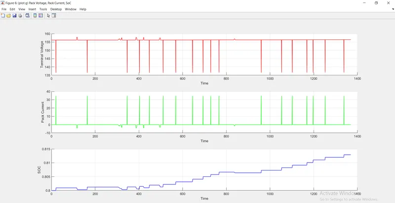
• (g) Plot of Pack current, Terminal Voltage and SoC

UDDS

HWFET

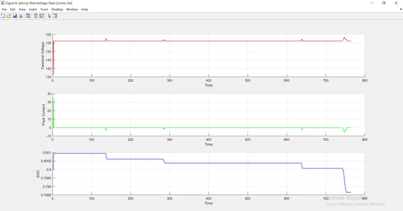
The above figures represents plot of Pack current, Terminal voltage and SOC. Pack current is the current or power generates by the electric motor due to regenerative braking at wheels of the vehicle. The amount of current power present in the battery is obtained by the State of Charge (SOC) parameter.This amount of charge is provided as the output Terminal voltage to run vehicle and its accessories at low speeds.

As discussed in previous plots we apply brakes at more number of times in city as compared to highway. So the UDDS cycle has more amount of charge generated as compared to HWFET cycle.

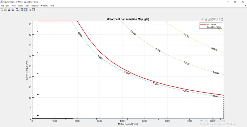
• (h) Plot of motor operating points on the motor input power map

UDDS

HWFET

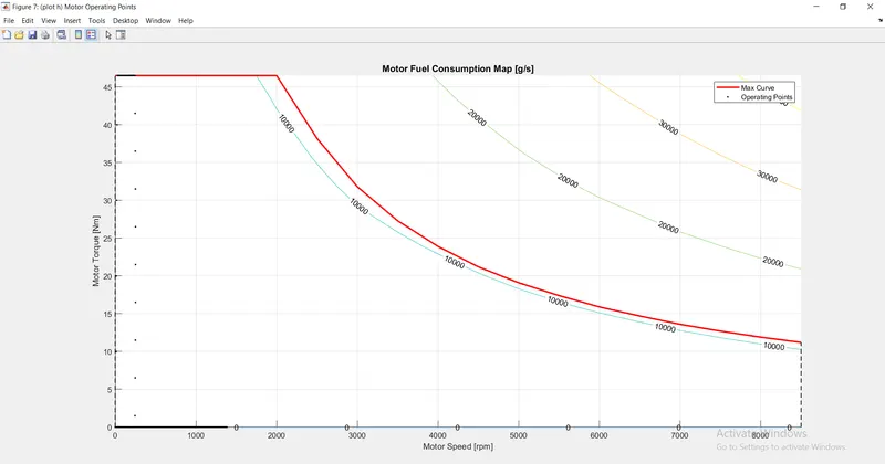
The above figures are the plot of Motor operating points vs Motor power map. The Red line indicates Max torque curve which represents high values at low speeds and decreasing further at high speeds. Black dots are motor operating points at perticular speed and torque.

CONCLUSION

Thus the above project contains the modeling or development of a forward energy-based fuel consumption model of a P1 hybrid vehicle using MATLAB and SIMULINK. As the model contains battery - the secondary power source we can see that the fuel economy values have increased as compared to conventional vehicle model.