Project 1
Project 1 - Model forward energy fuel consumption of a conventional vehicle
This project consists of modelling of forward energy fuel consumption of a conventional vehicle by using MATLAB and SIMULINK.
Conventional vehicle
All cars use some form of energy to make them move. In conventional vehicle this energy is provided in the form of gasoline or fuel. So in conventional cars that run on petrol or diesel, fuel and oxygen burn inside the engine to produce a small explosion. This explosion – known as internal combustion – pushes the pistons that make the wheels of the car move.
The conventional vehicle consists of many components that palys role in moving the vehicle. But the vehicle or this components can be grouped into three main parts containing the rest of the components in them. The three main components are, Driver, Controller and Powertrain.
1) Driver
A driver model is proposed that represents the driver’s decision-making process during the interaction between driver and vehicle and during the transition of driving tasks. The model includes the sensory perception process, decision-making, and motor response. The decision-making process during the interaction deals with the cognitive and emotional states of the driver. The driver obtains information about the automated system from inside the vehicle and also information about the traffic condition from outside the vehicle. This information can contain useful data about the driving situation that can help the driver with the driving task or decision making, and it also contains useless data that causes in disturbances and distracts the driver from the driving scene. Driver then provides this input signals to controller resulting in desired actions to be performed.
2) Controller
The controller is the main part of the loop that defines the control law for regulating the driver. The feedback controller is supposed to regulate the driver state to achieve the desired state (target state) so that driving becomes safer and the driver has comfortable driving experience. The controller is responsible for considering the situation and selecting the proper interaction strategy. As input, the controller obtains the driver state, the target state, the automation level, and the situation criticality.
3) Powertrain
- Engine: As the heart of your vehicle, an engine generates power to drive the car. An engine consists of pistons that move up and down inside cylinders and a crankshaft that translates the reciprocating motion into a rotating motion.
The engine is designed accordingly to meet the dsired requirements considering weather conditions, speed and power outputs, field of use, etc. There are various engine operating cycles designed and developed by different countries considering suitable factors like whether conditons, traffic condition, speed and weight parameters. Engine is developed according to this standerds of cycle. The different cycles are as follows;
i) UDDS - Urban Dynamometer Driving Schedule (called the "LA4" or "the city test" and represents city driving conditions)
ii) HWFET - Highway Fuel Economy Driving Schedule (represents highway driving conditions under 60 mph)
iii) NYCC - New York City Cycle (features low speed stop-and-go traffic conditions)
iv) The Japanese 10 Mode and 15 Mode Cycle
- Transmission: A transmission is a basic component in your car that makes sure the proper amount of power is transmitted to the wheels. Like a car's gearbox, the transmission takes the power from the engine and adjusts it according to driving conditions, ultimately transferring it to the wheels.
- Differential: A differential is a part of the rear axle. It allows each rear wheel to turn at a different speed. For instance, the differential is important when turning a corner, as the outside wheel needs to rotate faster than the inside wheel.
- Wheels: The power or energy generated by the engine is transmitted to the wheels for movement of vehicle. But the total energy generated by the engine can not be fully transfered to the wheels, this energy is also consumed to run the components in betwwen the engine and wheels. These components takes the energy from engine to wheels. As per calculations and reports, wheels get only 16% to 25% of the energy generated by engine. this energy is lost in the form of heat and friction in running and applying brakes of the vehicle.
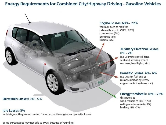
The powertrain is crucial because without the system working properly, your vehicle cannot move forward. To sum up, it's a group of parts that generate, convert, and consume energy to thrust your vehicle into motion.
Thus the driver can be considered as the user, powertrain as the body, and controller as brain of vehicle.
The powertrain can be modelled as Forward-facing model and Backward-facing model which can be satated as follows;
Forward facing model
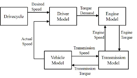
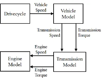
In this project, a typical midsize car with a 1.9L engine and a 4-speed automatic transmission is considered. Data of Time and Velocity is taken from ADVISOR data base developed by NREL, US EPA.
As discussed the three main components of vehicle are driver, controller and the powertrain, so these components can be modelled as simulink blocks as shown in below picture.
SIMULINK MODEL
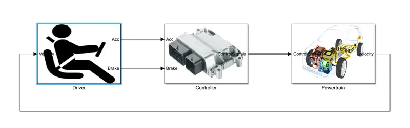
The above figure represents 3 blocks connencted to each other in the forwaed direction. The direction of connection also represents the path of information or signals transferred from one block to the other. The driver reads the speed of the running vehicle as input and accordingly gives the acceleration or brake to the vehicle. Controller takes acceleration and brake as input signals from driver and send this signals to powertrain. Powertrain recieves this signal and performs the required output actions.
The driver block also contains various components for reading and sending the signals. This can be seen in the below picture of driver model built inside the driver block.
Driver model
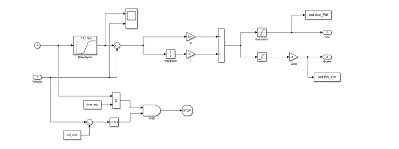
A driver model is a mathematical model which replicates the functionality of a driver like controlling, monitoring and stabilizing avehicle during various maneuvers. Driver models reproduce human actions or behavior to control the vehicle. The driver model consists of PID controllers outputting a generalised force, controlles speeds and an averaged steer angle to the steered wheels.
Controller model
The controller is responsible for considering the situation and selecting the proper interaction strategy. As input, the controller obtains the driver state, and produces the desired amount of power, torque, and fuel. It also controls the brake torque and transmission gear and desired temperature. The vehicle Controller includes an action to control fuel–air mixture that in turn produces the engine accelerator command. The inputs to this action include the Accelerator Cmd from the Driver and Engine Parameter such as revolutions per minute (RPM) and engine temperature.
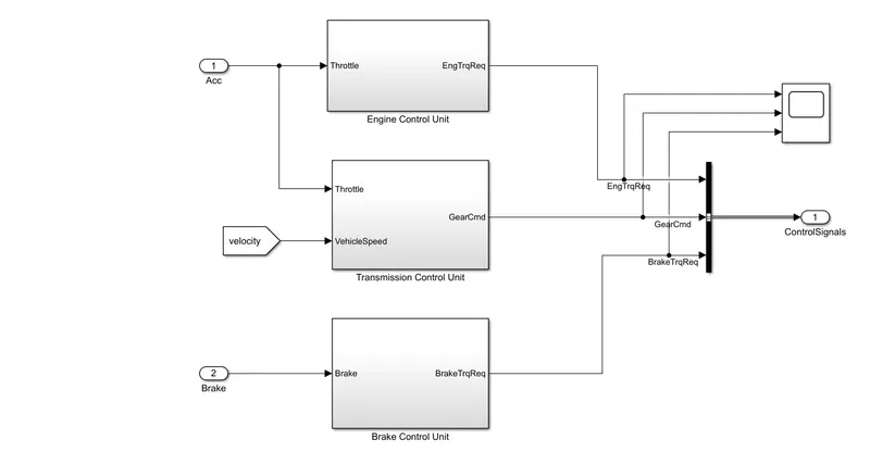
As shown in above figure the controller model consists of 3 sub control units namely, Engine control unit, Transmission control unit and Brake control unit. Each one of them can be discussed as follows.
- Engine control unit:
The controller takes in the acceleration from driver and is feed to Engine control unit and transmission unit. The engine control unit can be modelled as below.
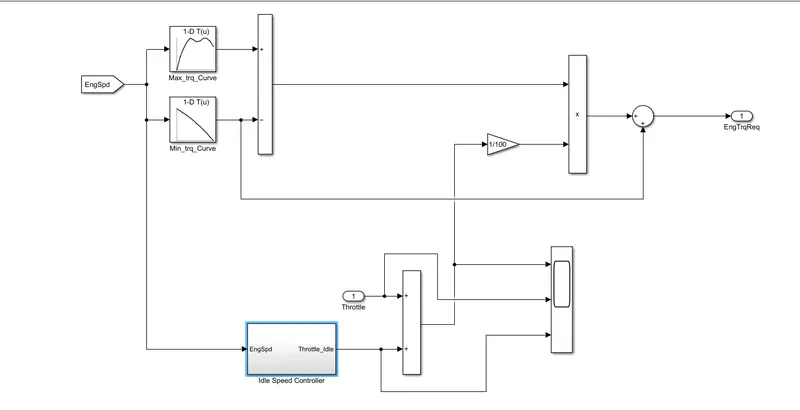
We can see that the engine control unit has an idel speed controller which makes sure that the engine is idling and does not go below the idle speed. The idle speed controller is again a PI controller having different gain values. This idle speed controller is then added to throttle which then converted to engine torque based in the max and min curve values.
- Transmission control unit:
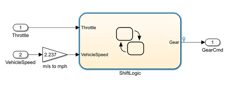
The Transmission control unit is built using Statespace as shown in the above picture.
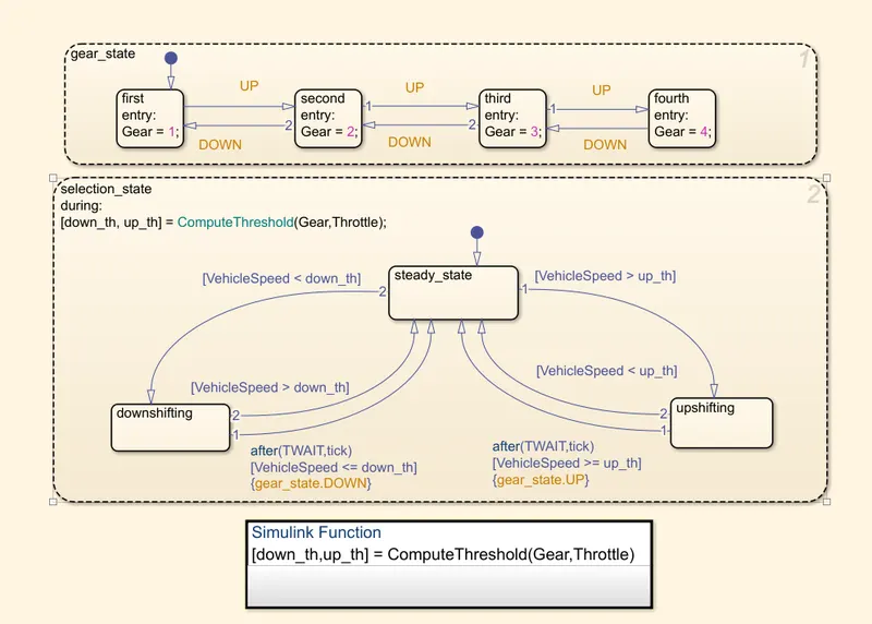
The model consists of a shiftlogic block having two different ststes namely, (i) gear state, and (ii) selection state. The gear state consists of different states having different transitions showing the switching of one state to other. The states represents up and down shifting of gears with respect to the speed of vehicle.
The calculations of this up and down shifting of gears are obtained from selection state and simulink function mentioned in above figure.. The state computes Threshold by taking gear and throttle as input and gives output as up and down.
- Brake control unit:
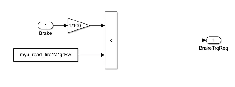
The input to this unit is brake peddle from 0 to 100% and it is combined with tyre friction or rolling friction. This value can be maximum or minimum depending ypon the vehicle speed, weight and rolling radius at the wheels. So the product of this values gives the brake torque at the output.
Now all the 3 sub control units go into the bus creater and gets combined giving signal outputs.
Powertrain
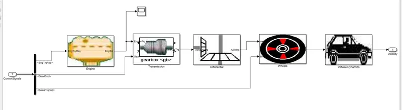
Powertrain is the source of power generation in the vehicle. It is the most important unit of vehicle which regulates the performance of the vehicle. A good quality powertrain is a key to a better operating range, acceleration, and top speed. So, when you accelerate your car from a standstill and feel a push of your engine power, just know that your powertrain propelled your vehicle.
These days, the importance of the Powertrain Control Module (PCM) has been recognized for its role in improving fuel economy and responding to global environmental regulations by controlling exhaust emissions. Thus, it is like the main computer of your car that controls fuel delivery, emissions functions, and many others. It also affects your engine's performance and drivability significantly.
As seen in the above figure, powertrain consists of various components like, Engine, Transmission, Differential, Wheels and Vehicle dynamics. Powertrain takes the control signals from the controller and pass this signals to above appropriate components according to their functions. Let us discuss the models and functionality of these components.
- Engine model
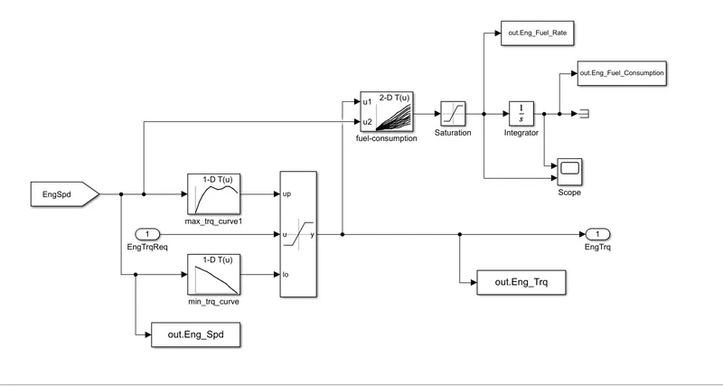
The engine model uses the map based model to model the fuel consumption of the engine. The model also consists maps for emmisions represented as engine max torque curve and engine min torque curve. Engine takes the torque request from controller and checks whether the torque is between max value or min value and based on that it is going to saturate the torque with the help of dynamic saturation block giving engine torque as output.
The Fuel consumption map takes this engine torque and Engine speed as input and gives fuel consumption data in grams/sec as output. The fuel consumption is then saturated to limit it less than zero.
- Transmission model
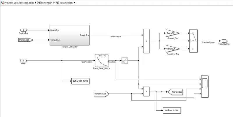
The output of engine torque goes to the transmission model and then it passes to torque converter blockas shown in above picture. The torque converter block has the engine dynamics block which calculates the acceleration ans speed of the engine based on the transmission speed and net torque acting on the engine.
Transmission block also has second input as gear controller which controls the gear ratio or shifting of gears based on speed.
- Differential model
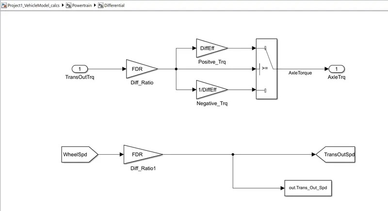
Input to the differential is the transmission output. This transmission output torque is then multiplied to Final Drive Ratio resulting in the axial torque. Differential also has the efficiency depending upon the positive torque or negative torque. Al this three terms is then feed to switch block to meet the required condition. The switch block will have a condition and if this condition satisfies it will allow the 1st path as output or else the 3rd path. Here if the product of torque and FDR is greater than equal to the positive torque then the axial torque will less than actual torque.
- Wheel model
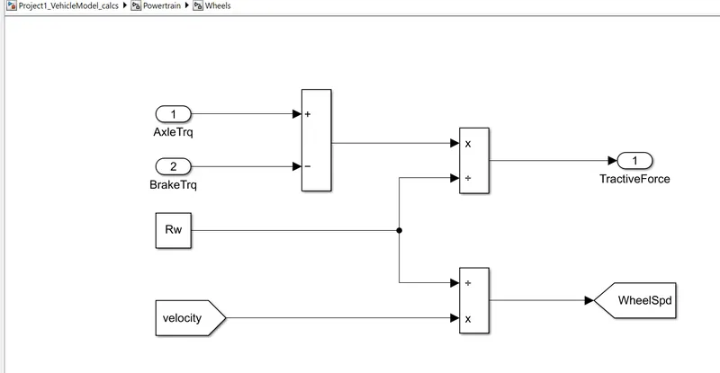
Wheels has two input values axle torque and brake torque as shown in above picture. Wheels has the brakes which retards the axle torque, giving the net torque output. The net torque is then divided to the rolling radius of the wheels resulting in the tractive force. The wheel speed can also be obtained by dividing the velocity to rolling radius as shown in above figure.
- Vehicle dynamics model
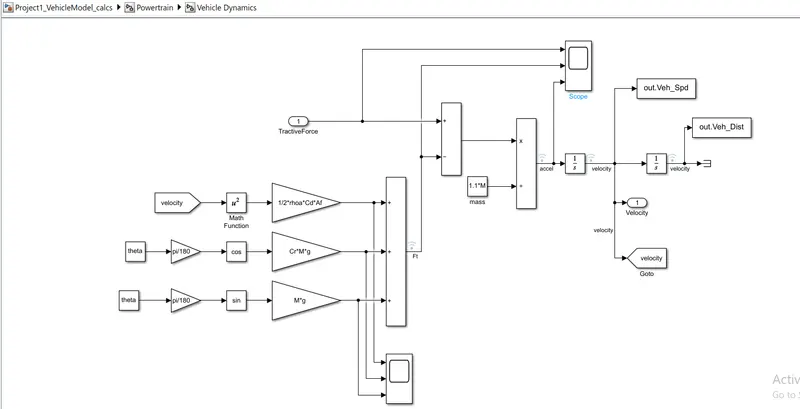
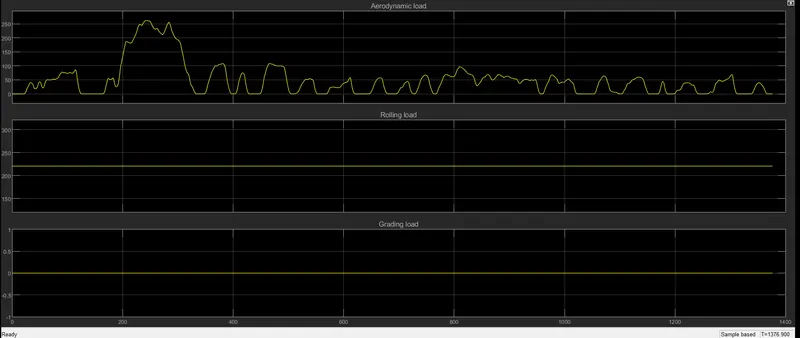
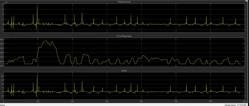
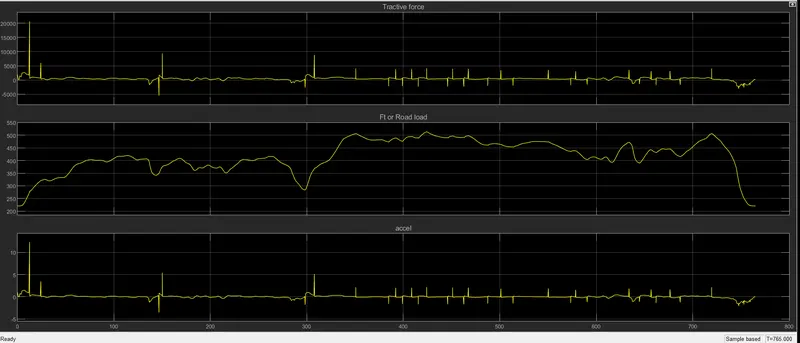
The vehicle dynamics block detects the vehicle velocity or speed based on what would be the input engine torque, tractive force and road load conditions. As shown in above figure the tractive force is feed from the wheels which is then substracted to the road load forces. This tractive force and road load is then divided by mass of the vehicle giving acceleration, velocity and distance of the vehicle.
The tractive force and road load can be calculated as follows;
M(dVveh/dt) = (ηtλtot/Rw)*Tm - (1/2*rhoa*A*Cd*(Vv+Vw)^2) + CrMgcosθ + Mgsinθ
where,
M = mass of vehicle in kg
Cd = drag coefficient
Af = frontal area of vehicle in m^2
ρ = air density in kg/m^3
Cr = rolling resistance
g = gravity
θ = grading angle or slope
r = radius of tyre
Vveh = vehivle velocity
Vwind = velocity of wind
The below mentioned file is a matlab script containing list of parameters to be cinsidered in the vehicle model and calculations. The file also consists commands for selection of cycle values from appropriate location. Calculations and plots of a forward conventional vehicle running on UDDS and HWFET cycles using MATLAB and SIMULINK is created below. The "if else" loop is used having 1 to 6 numbers representing each cycles for selection.
%%%%%%%%%%%%%%%%%%%%%%%%%%%%%%%%%%%%%%%%%%%%%%%%%%%%%%%%%%%%%%%%%%%%%
%% Skill-Lync -> Hybrid Drives Development
% Project 1 - Conventional Vehicle Model
% By - Deep Makwana
% Description: The project consists of modelling a forward energy based
% fuel consumption conventional vehicle running on two different engine
% operating cycles. Below matlab script file consists the list of
% parameters that are involved in calculations of force, power and energy
% required to run the vehicle. The selection of cycle is based on the
% matlab commands as mentioned below.
%% Initialization File
% Initialization file for loading the variables for the Conventional vehicle simulation model
%% Vehicle Parameters
M = 1500; % Vehicle weight [kg]
Cr = 0.015; % Rolling resistance coefficient
Rw = 0.35; % Rolling radius [m]
Cd = 0.33; % Drag coefficient
Af = 2; % Frontal area [m2]
rhoa = 1.225; % Air density [kg/m3]
Vwind = 0; % Wind velocity [kmph]
g = 9.81; % Gravitational acceleration [m/s2]
theta = 0; % Slope [deg]
myu_road_tire = 1; % Coefficient of friction between tire - road interface
%% Powertrain Parameters
FDR = 3.73; % Final Drive Ratio / Diff Ratio
DiffEff = 0.99; % Differential efficiency (assumed independent of operating conditions)
NumGear = 4; % Number of gears in transmission
TransGear = [1:NumGear]; % Transmission Gears
TransRatio = [3.06, 1.62, 1, 0.7]; % Corresponding Transmission ratios
TransEff = 0.90; % Transmission efficiency (assumed independent of operating conditions)
TC_SR = [0, .5, .6, .7, .8, .87, .92, .94, .96, .97, 1]; % Torque Converter Speed Ratio (Matlab default) -> TurbSpd/PumpSpd
TC_TR = [2.232, 1.5462, 1.4058, 1.2746, 1.1528, 1.0732, 1.0192, 1, 1, 1, 1]; % Torque Converter Torque Ratio (Matlab default) -> TurbTrq/PumpTrq
TC_Cf = 1e-4 * [.72558, .66322, .63463, .59042, .51331, .4144, .29287, .22444, .12186, .04386, 0]; % Torque Converter Capacity Factor (Matlab default) -> PumpTrq/PumpSpd^2 [Nm/rpm^2]
load Project1_Files/Vehicle_Data/Engine_data_1_9L_Saturn_95kW
load Project1_Files/Vehicle_Data/Trans_Shift_map
%% Driver Parameters
Kp = 10; % P gain for driver PI model
Ki = 1; % I gain for driver PI model
Drive_Cycle_Select = 1; % Drive cycle selection
% Drive cycle values in m/s
if Drive_Cycle_Select == 1
load Project1_Files/DriveCycles/UDDS;
elseif Drive_Cycle_Select == 2
load Project1_Files/DriveCycles/HWFET;
elseif Drive_Cycle_Select == 3
load Project1_Files/DriveCycles/FTP;
elseif Drive_Cycle_Select == 4
load Project1_Files/DriveCycles/US06;
elseif Drive_Cycle_Select == 5
load Project1_Files/DriveCycles/NEDC;
elseif Drive_Cycle_Select == 6
load Project1_Files/DriveCycles/WLTP;
end
time_end = cyc_time(end);
vel_end = cyc_vel(end);
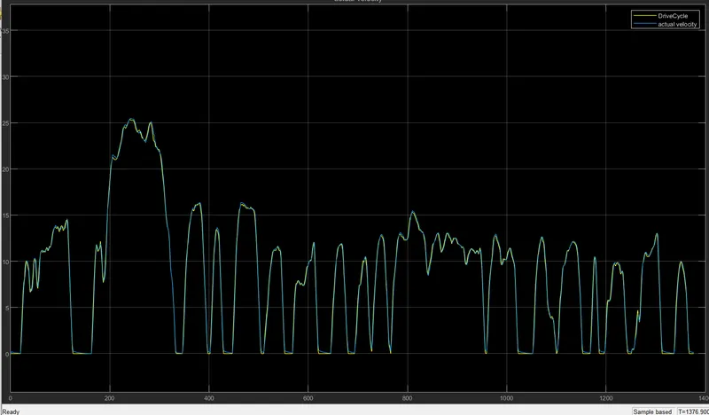
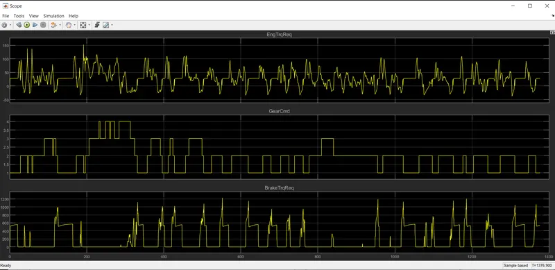
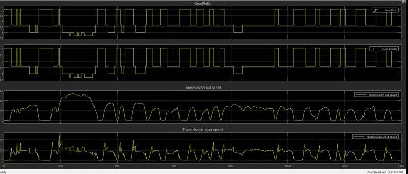
After running the above matlab script the list of parameters will be stored in the workspace and these values will be read by the simulink models as per stated. Now the simulink model is also runned and the outputs are also stored in workspace. Different plots obtained from the simulink model can be represented as below.
1. UDDS cycle scope plots
Driver : Drive cycle & velocity
Controller : Engine torque, Transmission gear, and Brake torque
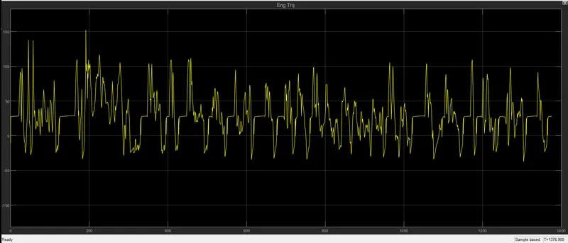
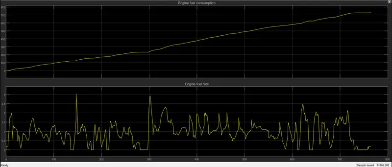
Engine : Engine Fuel Rate & Fuel Consumption
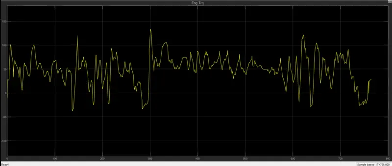
Engine torque
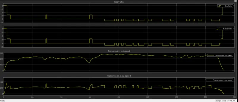
Transmision : Gear ratio, trans. input, tans output
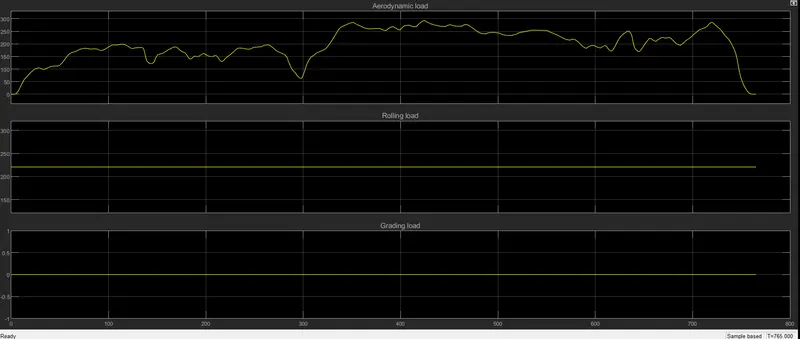
Vehicle dynamics : Road loads
Vehicle dynamics : Tractive force, road load and accel.
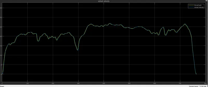
2. HWFET cycle scope plots
Driver : Drive cycle & velocity
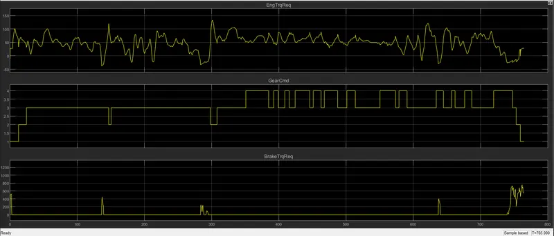
Controller : Engine torque, Transmission gear, and Brake torque
Engine : Engine Fuel Rate & Fuel Consumption
Engine torque
Transmision : Gear ratio, trans. input, tans output
Vehicle dynamics : Road loads
Vehicle dynamics : Tractive force, road load and accel.
The below script file is the post-procesing file and consists the commands used to plot various parameters, compare and observe the behaviour of the vehicle while moving or steady conditions.
%%%%%%%%%%%%%%%%%%%%%%%%%%%%%%%%%%%%%%%%%%%%%%%%%%%%%%%%%%%%%%%%%%%%%
%% Skill-Lync -> Hybrid Drives Development
% Project 1 - Conventional Vehicle Model
% By - Deep Makwana
% Description: A MATLAB script is Created to analyse data and to generate plots.
% Here we rename the variables loaded from the model,
% do some basic post-process calculations and generate results and plots.
% The following file is to used with the Initialization file and Simulink
% results for post-processing of the data.
% The file is incomplete, has some examples of how the data is imported
% into a readable format, data analysis and plotting examples.
% Based on the project task, use commands in a similar format as given
% below, to analyse the data and generate required plots.
% You can change variable names if desired
%% Post-Processing File
% File for post-processing the Conventional vehicle simulation model data
%% Renaming variables
Time = out.tout;
Acc_Pdl = out.Acc_Pdl; % Accelerator pedal [%]
Brk_Pdl = out.Brk_Pdl; % Brake pedal [%]
Gear_Cmd = out.Gear_Cmd; % Transmission gear
Trans_In_Spd = out.Trans_In_Spd*30/pi; % Transmission input speed [rpm]
Trans_Out_Spd = out.Trans_Out_Spd*30/pi; % Transmission output speed [rpm]
Eng_Trq = out.Eng_Trq; % Engine brake torque [Nm]
Eng_Spd = out.Eng_Spd*30/pi; % Engine speed [rpm]
Eng_Fuel_Consump = out.Eng_Fuel_Consumption; % Engine fuel consumption [g]
Veh_Dist = out.Veh_Dist/1000; % Distance traveled by vehicle [km]
Veh_Spd = out.Veh_Spd*18/5; % Vehicle speed [kmph]
%% Data Analysis
Eng_Pwr = (Eng_Spd*pi/30).*(Eng_Trq/1000); % Engine brake power [kW]
rho_petrol = 0.7197; % Density of petrol [kg/L]
kmpl = Veh_Dist(end)/(Eng_Fuel_Consump(end)/1000/rho_petrol); % Fuel economy [kmpl]
%% Plotting vehicle characteristics time trace
figure('Name','vehicle characteristics time trace')
subplot(3,1,1)
hold on
grid on
plot(Time, Acc_Pdl, 'linewidth', 1, 'Color', 'black');
plot(Time, Brk_Pdl, 'linewidth', 1, 'Color', 'red');
ylabel('Pedal [%]')
xlim([0, Time(end)]);
legend('Accel','Brake');
subplot(3,1,2)
hold on
grid on
plot(Time, Trans_In_Spd, 'linewidth', 1, 'Color', 'black');
plot(Time, Trans_Out_Spd, 'linewidth', 1, 'Color', 'red');
ylabel('Speed [rpm]')
xlim([0, Time(end)]);
ylim([0, 6000]);
legend('Trans Input','Trans Output');
subplot(3,1,3)
hold on
grid on
plot(Time, Gear_Cmd, 'linewidth', 1, 'Color', 'black');
xlim([0, Time(end)]);
xlabel('Time [s]');
ylabel('Gear');
%% Plotting engine operating points on engine fuel map
figure('Name','Engine Operating Points');
hold on
grid on
title('Engine Operating Points','fontsize',12);
p1=plot(Eng_map_spd*30/pi,Eng_max_trq,'linewidth',2,'color','r');
p2=line([Eng_map_spd(end)*30/pi Eng_map_spd(end)*30/pi],[0 Eng_max_trq(end)]);
set(p2,'linewidth',1,'linestyle','--','color','k');
p3=line([Eng_map_spd(1)*30/pi Eng_map_spd(1)*30/pi],[0 Eng_max_trq(1)]);
set(p3,'linewidth',1,'linestyle','--','color','k');
[c,h] = contour(Eng_map_spd'*30/pi,Eng_map_trq,Eng_fuel_map');
clabel(c,h);
xlabel('Engine Speed [rpm]');
ylabel('Engine Torque [Nm]');
title('Engine Fuel Consumption Map [g/s]');
p4 = plot(Eng_Spd,Eng_Trq,'.','color','k');
legend([p1 p4],{'Max Curve','Operating Points'});
axis([Eng_map_spd(1)*30/pi Eng_map_spd(end)*30/pi 0 Eng_map_trq(end)]);
%% (c) Plotting engine torque, engine power, fuel rate, fuel comnsumption.
figure('Name','Engine torque,power,fuel rate, fuel conp.');
subplot(4,1,1)
hold on
grid on
plot(Time, Eng_Trq,'b','linewidth',1); xlabel('Time'); ylabel('Torque')
subplot(4,1,2)
hold on
grid on
plot(Time, Eng_Pwr,'r','linewidth',1); xlabel('Time'); ylabel('Power')
subplot(4,1,3)
hold on
grid on
plot(Time, Eng_Fuel_Consump,'k','linewidth',1); xlabel('Time'); ylabel('Fuel consumption')
subplot(4,1,4)
hold on
grid on
plot(Time, Eng_fuel_rate,'g','linewidth',1); xlabel('Time'); ylabel('fuel rate')
%% (b) Plotting of time trace for engine, transmission input, transmission output and wheel speed
figure('Name','Engine torque, Trans. in, Trans. out, wheel speed');
hold on
grid on
plot(Time, Trans_In_Spd,'b','linewidth',1);
plot(Time, Trans_Out_Spd,'y','linewidth',1);
plot(Time, Veh_Spd,'g','linewidth',1);
xlabel('Time (s)')
ylabel('speed (rpm)')
legend('Trans input','Trans output','Wheel speed');
After running the above script various plots and results obtained are mentioned below.
a). Fuel economy for UDDS - 13.6312 kmpl
Fuel economy for HWFET - 16.3072 kmpl
As UDDS cycle belongs to the city driving conditions the fuel economy of this cycle will be less than HWFET cycle. The reasons behind less economy is the uneven road conditions resulting in frequent braking and accelerating the vehicle, more traffic and signal conditions in city resulting in idling of vehicle etc. Whereas the HWFET belonging to highway driving conditions has better road conditions, very less traffic and no signals resulting in more fuel economy.
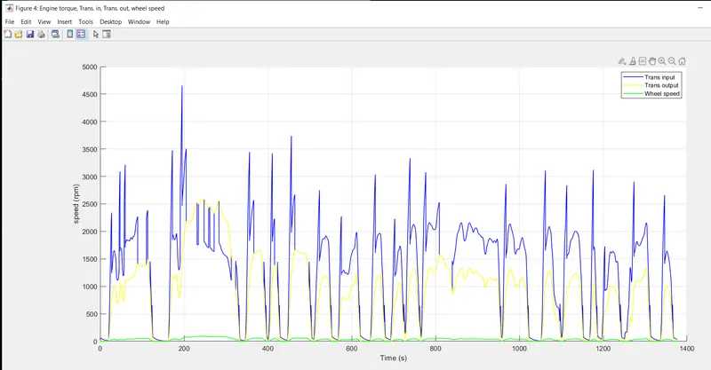
b). Plot the time trace for engine, transmission input, transmission output and wheel speed on one plot.
plot for UDDS
plot for HWFET
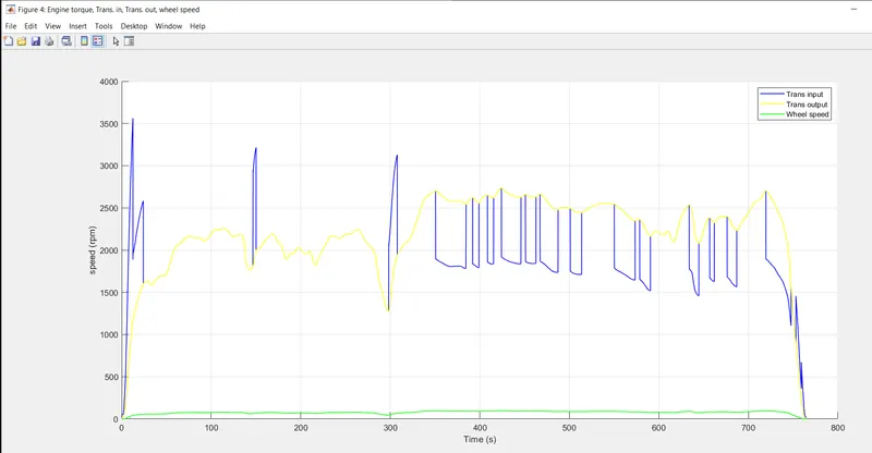
We can see from the plots that the values of transmission input and transmission output speed/power is high and values of wheel speed is low. The reason behind it is the power consumed by the components in transmission and various losses occured in transmitting the energy from engine to wheels.
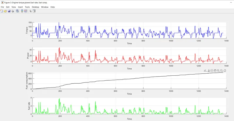
c). Plot engine torque, engine power, fuel rate and fuel consumption using subplots.
plot for UDDS
plot for HWFET
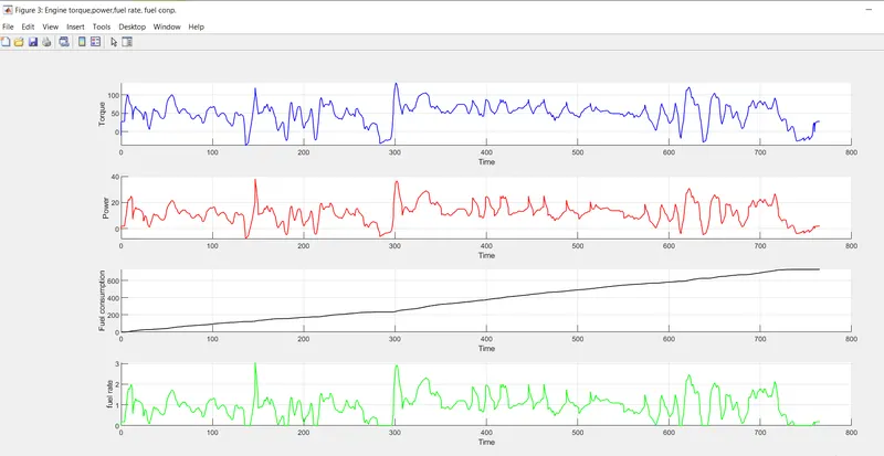
The torque requirements of the drive cycle are different, so the fuel flow rate varies and fuel consumption is calculated. The HWFET drive cycle has higher power and torque requirements and less negative torque and power.
d). Plot accelerator and brake pedal, gear command, vehicle desired and actual speed, vehicle distance using subplots.
plot for UDDS
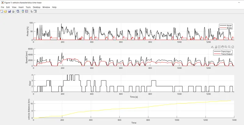
Acceleration and brake pedals are used more because the drive cycle is not very smooth and the gear has to be shifted frequently.
plot for HWFET
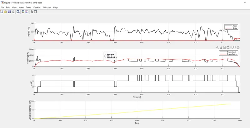
Brake requirements are lower, more accelerator pedals are applied on the highway drive cycle, and gear shifts often occur because the drive cycle is smoother. Acceleration and brake pedal, the gear command of the transmission control unit, the required speed of the vehicle, the actual vehicle speed and the actual vehicle distance are plotted.
e). Plot the engine operating points on the engine fuel map.
plot for UDDS
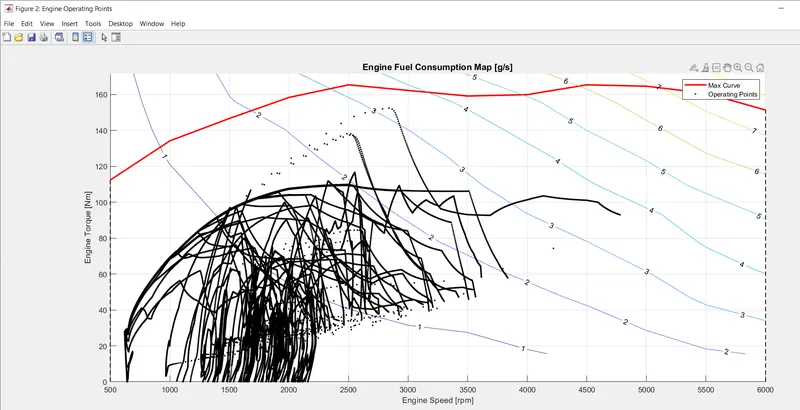
plot for HWFET
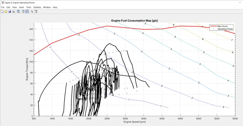
The engine operating points are plotted on the fuel map and the operating point is under the maximum torque curve.