Project 2
Project 2 final Report;
AIM;
- Development of a forward energy-based fuel consumption model of a P1 hybrid vehicle.
- Quantify the improvement in fuel economy numbers for the hybrid vehicle [kmpl], compared to the conventional vehicle, on the urban cycle [UDDS] and highway cycle [HWFET].
- To analyze and understand the vehicle operating points in terms of engine and motor speed, torque, transmission speeds, pedal positions, gear, distance traveled, battery voltage, current, SoC etc.
- Write pre-processing scripts in MATLAB to load all the variable needed to run the simulink model.
- Modify conventional vehicle simulink model into a hybrid vehicle model.
- Analyze data and write post-processing scripts in MATLAB to create plots using MATLAB scripts.
OBJECTIVES;
- Tabulate the fuel economy numbers [kmpl] for UDDS and HWFET cycle. Compare these numbers with the baseline numbers for conventional vehicle model.
- Plot the time trace for engine, transmission input, transmission output and wheel speed on one plot.
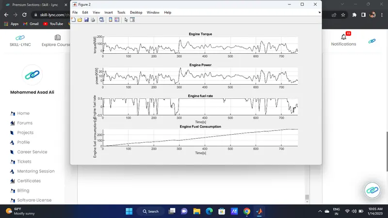
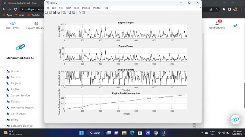
- Plot engine torque, engine power, fuel rate and fuel consumption using subplots.
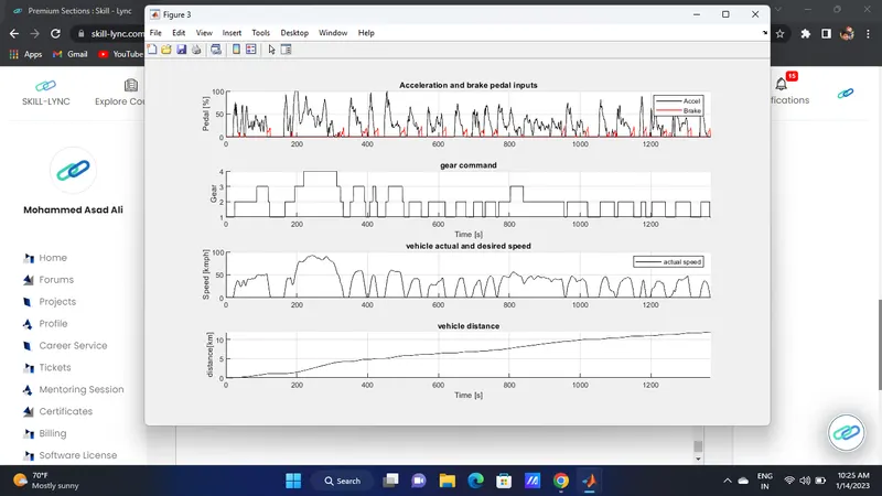
- Plot accelerator and brake pedal, gear command, vehicle desired and actual speed, vehicle distance using subplots.
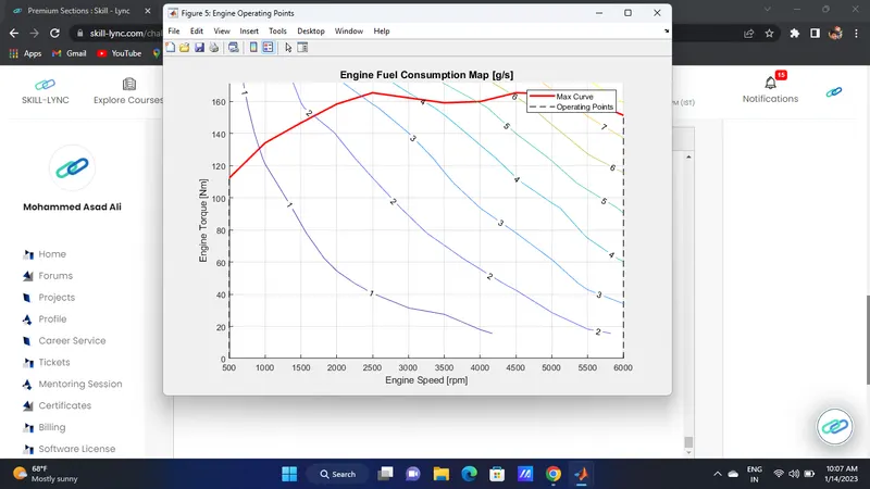
- Plot the engine operating points on the engine fuel map.
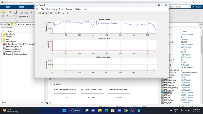
- Plot motor speed, torque, motor input power using subplots.
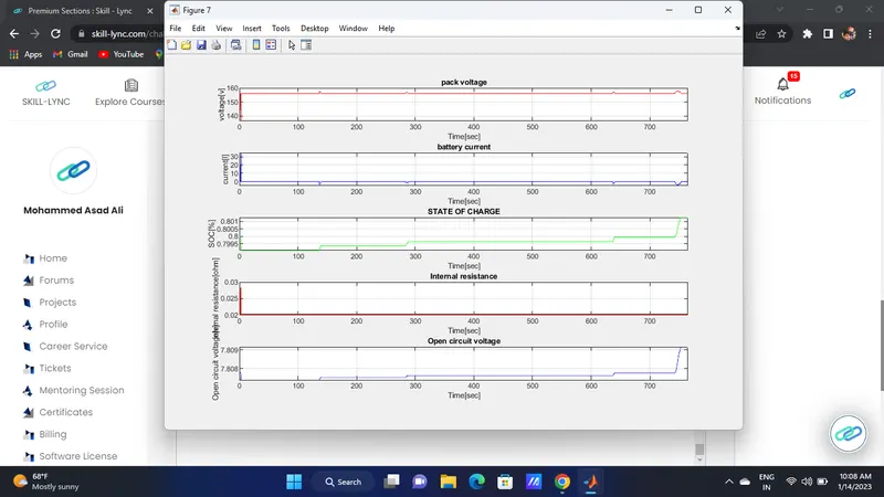
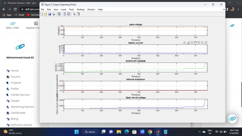
- Plot pack voltage, current and SoC using subplots.
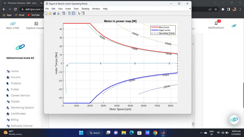
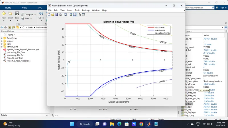
- Plot the motor operating points on the motor input power map, with the motor max motoring and generating torque curves.
- Write down appropriate brief comments on each of these plots, describing the vehicle behavior throughout the drive cycle.
- Generate the plots for both drive cycles
Theory;
Forward Model Approach;
- The forward modelling approach is also called as cause-effect,engine to wheel method.
- The direction of calculation is the same as the direction of positive power flow from engine to wheel.
- This approach is based on vehicle dynamics equation and the behaviour of each powertrain components and their dynamics interaction.
- In this we start with modeled using a ‘Driver' block, which is a basic PI controller that generates accelerator and brake pedal outputs to match the desired and actual vehicle speeds.
- The ‘Controller’ block is the brains of the vehicle, representing the electronic controls units. Based on the driver inputs, it generates desired engine torque, desired transmission gear and desired brake torque.
- These inputs are fed to the ‘Powertrain’ block which represents the drivetrain of the vehicle. It consists of an ‘Engine’ and 'Electric Motor throuth battery' connected to the ‘Automatic transmission’ through a ‘Torque Converter’. The output of the transmission is connected to the ’Differential’, which powers the ‘Wheels’, that provides the tractive force for vehicle acceleration. The longitudinal dynamics of the vehicle along with the road load is represented in the ‘Vehicle Dynamics’ block.
P1 Hybrid Vehicle Model;
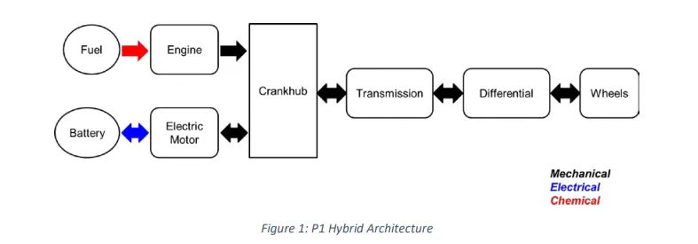
Vehicle Model;
Pre-Processing;
A MATLAB scripts has been created to load all the variable needed for running the Simulink model and for post-processing. The drive cycle selection is also done here. Before running the Simulink vehicle model, run this initialization script.
% Initialization file for loading the variables for the P1 Hybrid vehicle simulation model
Drive cycle can be selected from this MATLAB scripts by changing the variable Drive_cycle select to,
1
UDDS
2
HWFET
3
FTP
4
US06
5
NEDC
6
WLTP
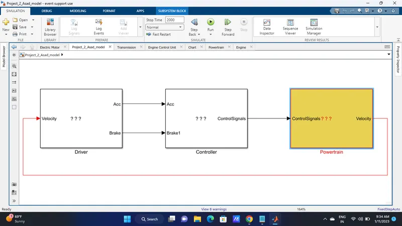
- Here we start with modeled using a ‘Driver model' block, which is a basic PI controller that generates accelerator and brake pedal outputs to match the desired and actual vehicle speeds.
- The ‘Controller model’ block is the brains of the vehicle, representing the electronic controls units. Based on the driver inputs, it generates desired engine torque, desired transmission gear and desired brake torque.
- These inputs are fed to the ‘Powertrain model’ block which represents the drivetrain of the vehicle. It consists of an ‘Engine model with Electric Motor’ connected to the ‘Automatic Transmission model’ through a ‘Torque Converter’. The output of the transmission is connected to the ’Differential’, which powers the ‘Wheels’, that provides the tractive force for vehicle acceleration. The longitudinal dynamics of the vehicle along with the road load is represented in the ‘Vehicle Dynamics model’ block.
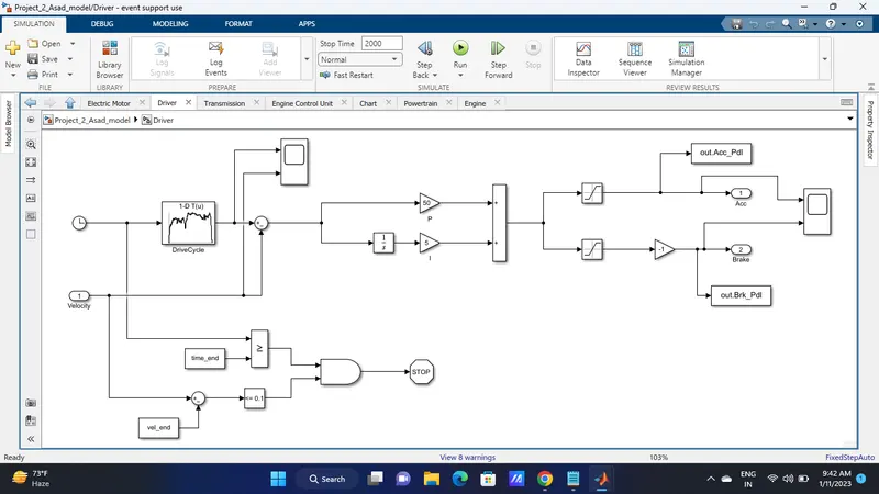
Driver Model;
- ‘Driver model' block, which is a basic PI controller that generates accelerator and brake pedal outputs to match the desired and actual vehicle speeds.
- The ‘Controller’ block is the brains of the vehicle, representing the electronic controls units. Based on the driver inputs, it generates desired engine torque, desired transmission gear and desired brake torque. These inputs are fed to the ‘Powertrain’ block which represents the drivetrain of the vehicle.
- a state flow machine is used to represent the supervisory control unit which decided the operating mode while its is start /stop mode or cruising mode or regen braking mode for each modes the engine drive and the motorr drive are controlled.
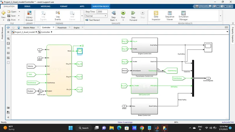
- the input to the state flow charts is accle. and brake pedal input from the driver unit engine actual speed actual vehicle speed soc status ant the clutch lockup stste and the output to the controller are the mode engine on /off request engine input thottle and electric motor input throttle.
- all control signal passed to transmission model which represent the drive train.
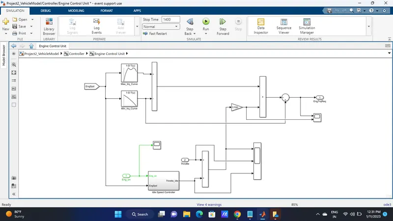
Engine control unit:
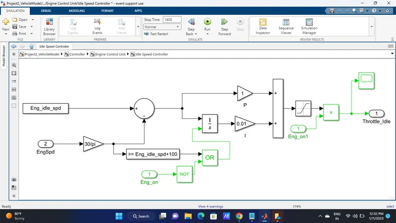
1. engine control unit compare engine speed with the maximum torque and minimum torque curve of the lookup table and give the required torque command to the engine block. the throttle input is combine with the idle speed throttle and gains with torque output from the lookup table to estimate the torque input required for the engine.
2. throttle input idle throttle and their sum can be scoped from this block.
Idle speed controller;
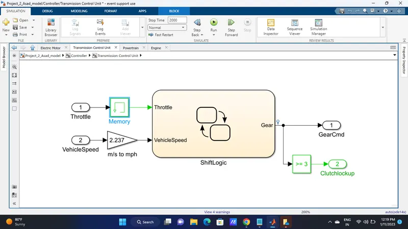
Transmission control block;
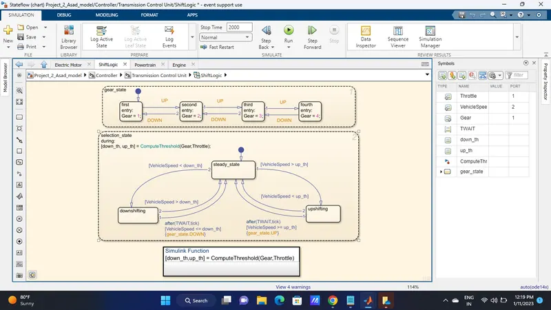
The transmission control block control the gear shifting using the study flow variable chart.
The gear shifting is controlled according to the vehicle speed and throttle input.
The gear command is passed to the transmission block to select the desired gear ratio.
Electric motor control unit;
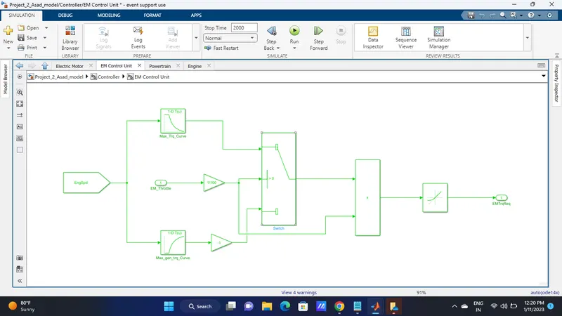
Motor control unit compare EM speed with the max torque curve and max torque generation curve of the lookup table and give the required torque command to the electric motor the EM throtle input is used to compare the lookup table and to estimate the torque input required for the e-motor.
Brake control unit;
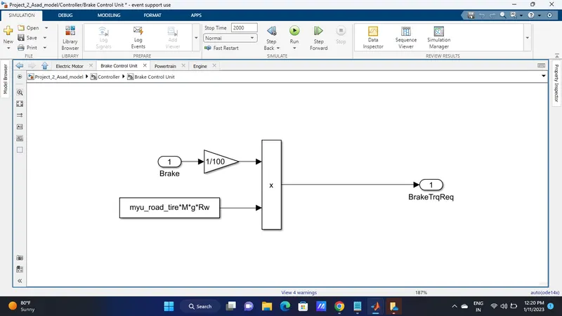
Brake control unit produce required brake torque according to the brake pedal input and passes the brake torque in to the wheel block in the transmission model.
Powertrain model;
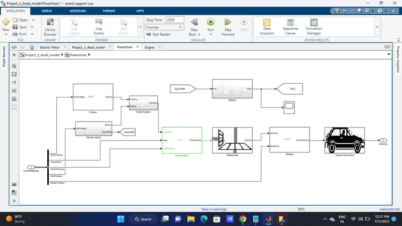
The power train model include all the components that converts the power of the engine into the vehicle motion.
This includes the engine,e-motor,battery pack,transmission,diffential,wheels,and vehicle body dynamics subsystem.
Battery model;
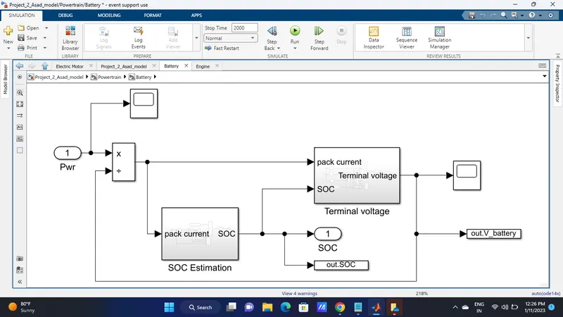
A battery pack subsystem is created with electric power input and battery soc as output
2 diff. subblock have been created to determine the soc and termonal voltage seperately soc is used to determine he terminal voltage.
SOC Estimation model;
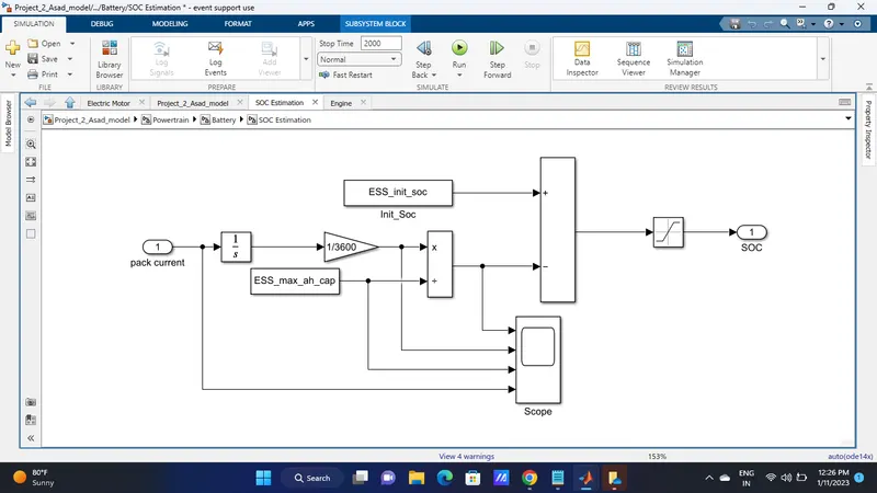
pack current in ampere is converted to amphr and divides with max capacity and adds with the initial soc to determine the soc of the battery at each instance the soc value is limited betwen 0 to 1.
Terminal voltage model;
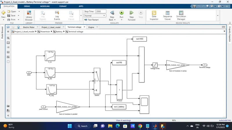
Ideal voltage and internal resistance are determined by 1D lookup table and battery voltage is determoned using the model.
The specified values are send back to workspace using the to workspace block and can be used for post processing.
Engine model;
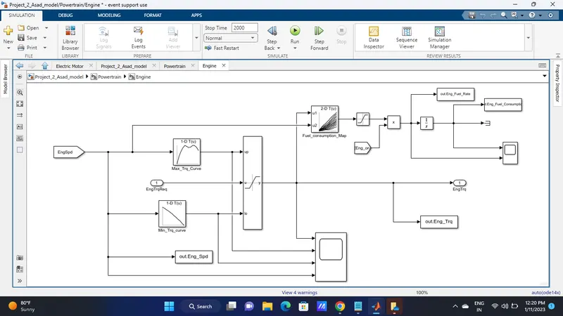
- Based on the engine speed the required torque from the controller is saturated between max torque curve and min torque curve and passes the engine torque to the transmission block
- The 2D lookup table is used to calculate the fuel flow rate based on engine speed and engine torque.
- The new engine also has an on/off feature to eliminate the fuel flow rate when the engine is off also the engine torque cannot be negative torque as min.torque curve mode saturated.
- The fuel rate is then integrated to find the fuel consumption.
- Estimated fuel flow rate fuel consumption engine torque and engine speed are passed to the MATLAB workspace using the to-workspace block
- Engine fuel flow rate and fuel consumption are scoped.
Electric Motor Model;
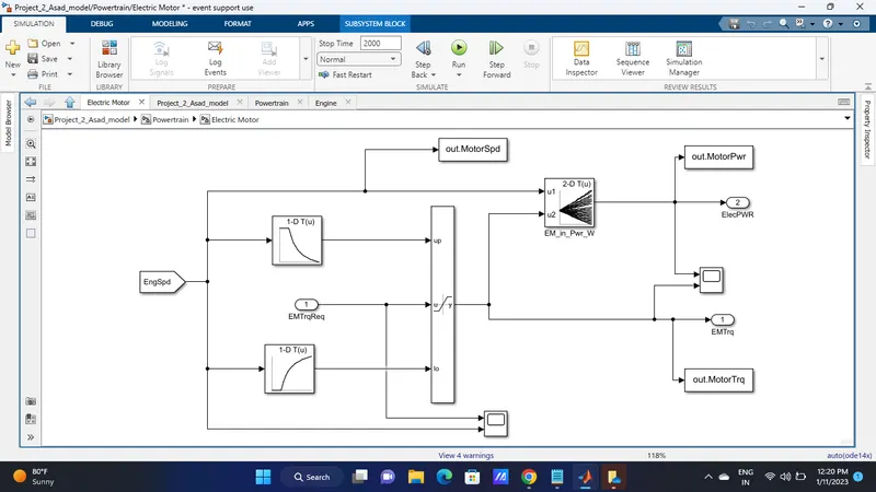
Based on the engine speed the required EM torque from the cotroller is saturated between max EM torque curve and max EM torque generation curve and passes the EM torque to the crank hub
the 2D lookup table is used to calculate the input electric power to the motor basd on the EM speed and EM torque.
crank hub;
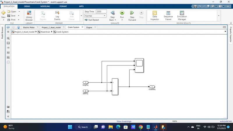
Crank hub adds up the EM torque and the engine torque and pass it to the transmission block as the crank torque.
Transmission model;
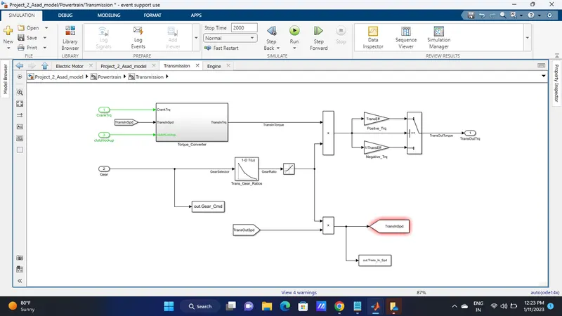
The engine block is connected to the automatic transmission via a torque converter the output of the transmission is connected to the differential.
Torque converter;
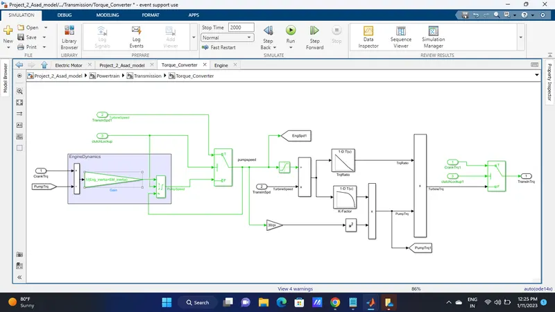
The gear selection from the transmission control unit is multiplied by the engine torque in this block and the efficiency and engine dynamics of the torque converter are applied in this model.
Differential Model;
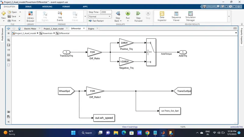
The transmission output torque is multiplied by the differential ratio and differential effieciency in this block and the torque is transmiteed to the wheel as the axle torque.
Wheel Model;
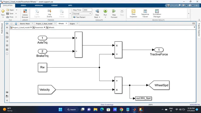
The brake torque from the control model is subtracted from the axle torque and divides from the rolling radius to determine the tractive force
The wheel speed is calculated from the vehicle velocity and saved in the workspace.
Vehicle dynamics;
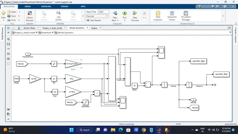
The longitudinal dynamics of the vehicle along with the road load is represented in the vehicle dynamics block
Tractive force and road loads are used to calculate the vehicle velocity
1. Tractive force = ηt*λt*Te/Rw = M*(dVveh/dt) + 0.5 *ρa *Af*Cd*(Vveh+Vwd)^2 + Cr*M*g*cosθ +M*g*sinθ
2. Road load = 0.5 *ρa *Af*Cd*(Vveh+Vwd)^2 + Cr*M*g*cosθ +M*g*sinθ
where,
ρa = air density
Af = frontal area
Cd = drag co-efficients
Cr = rolling co-efficients
M = vehicle mass
g = acceleration due to gravity
θ = slope
- The variable are loaded on the workspace using MATLAB scripts.
- The acceleration velocity and distance travelled are calculated and stored in the workspace.
Post processing file;
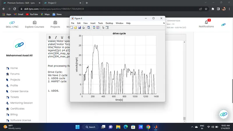
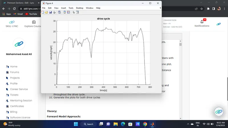
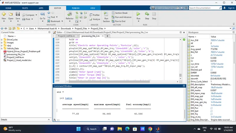
2. HWFET cycle.
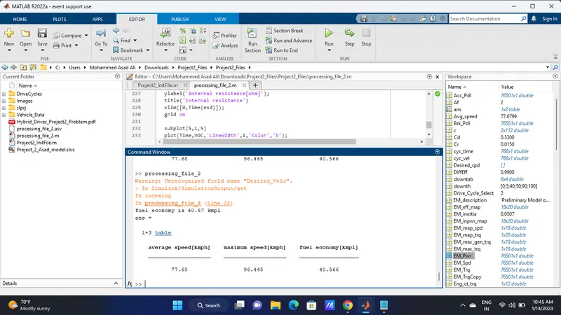
The time trace for engine ,transmission input,transmission output,wheel speed;
1. UDDS CYCLE;
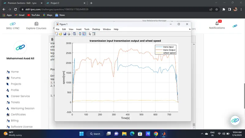
2. HWFET cycle.
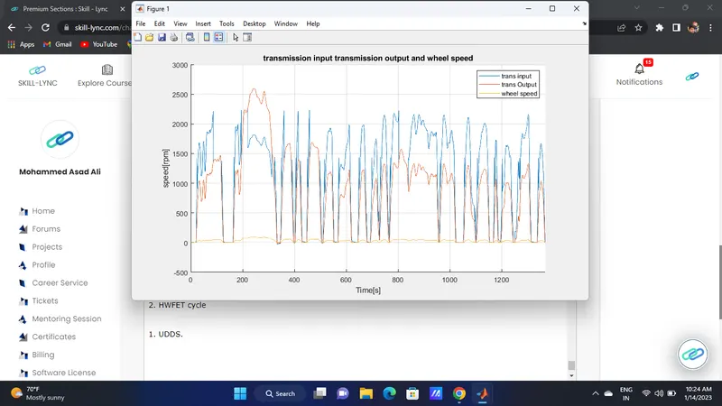
1. Much of the fluctuating input speed is facilitated by the torque convertor and the transmission input speed fluctuates according to the engine torque required to achive the drive cycle.
2. wheel speed and transmision output speed vary according to gear and differential ratio.
Engine torque,engine power,fuel rate,fuel consumption;
1.UDDS CYCLE;
2. HWFET cycle.
Accelerator and brake pedal,gear command,vehicle desired and actual speed,vehicle distance:
1.UDDDS CYCLE;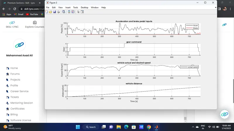
2. HWFET cycle.
1. Acceleration and brake pedals are used more bcoz the drive cycle is not very smooth and the gear has to be shifted frequently.
2. Brake requirement are lower more acceleretor pedal are applied on the highway drive cycle and gear shift often occurs bcoz the drive cycle is smoother.
3. Acceleration and brake pedal the gear command of the transmission control unit the required speed of the vehicle the actual speed and the actual vehicle distance are plotted.
The engine operating points on the engine fuel map;
1.UDDS CYCLE;
2. HWFET cycle.
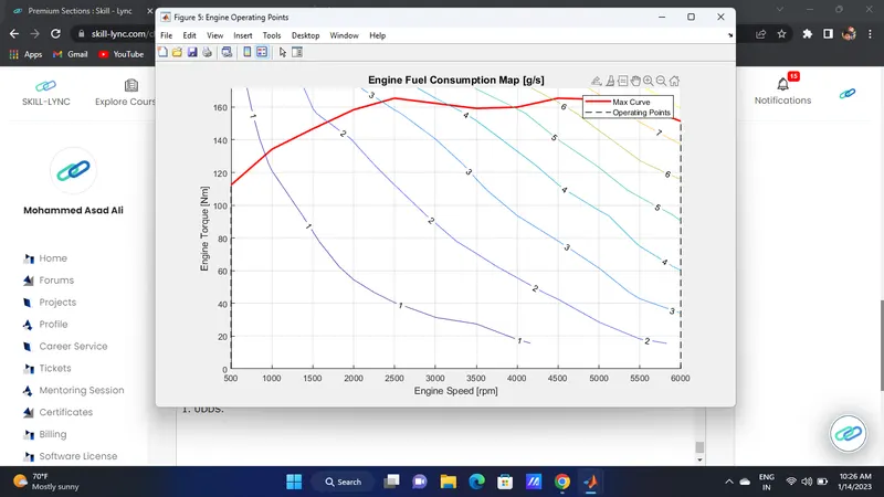
1. The engine operating points are plotted on the fuel map and the operating points is under the maximum torque curve.
The motor speed,motor torque,motor input power;
1. UDDS
2. HWFET cycle.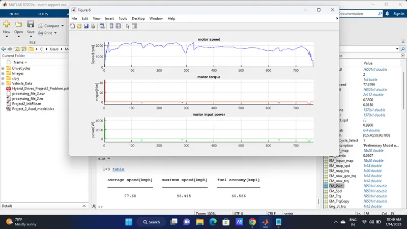
The pack voltage ,current,SOC, VOC,internal resistance;
1.UDDS
2. HWFET cycle.
The motor operating points on the motor inputs power map,with the motor max motoring and generating torque curves;
1. UDDS
2. HWFET cycle.
CONCLUSION ;
1. Therefor the forward energy based fuel consumption model of a P1 Hybrid vehicle has been successfully simulated using MATLAB and SIMULINK.Analysis and understand vehicle operating points based on engine.
2.Speed,torque,transmissionspeed,pedalposition,gear,distance,velocity,acceleration,battery,voltage,current,SOC and pedal position acceleration,battery,voltage,current,SOC and pedal position.
3. Post process calculation were performed and the required graphs were successfully plotted.
Succesfully calculated vehicle fuel efficiency number(kmpl) for the given city cycle UDDS and highway cycle HWFET.and also compared to the conventional vehicle.
Thank you,