Project 2
PROJECT NAME
The development of a forward energy-based fuel consumption model of a P1 hybrid vehicle.
PROJECT AIM
- Build a Simulink model using blocks and complete the vehicle Model
- Write scripts in MATLAB to load all the variables needed to run the simulation model.
- Analyze data and create plots using MATLAB scripts.
PROJECT OBJECTIVE
- Tabulate the fuel economy numbers (kmpl) for UDDS and HWFET cycles. Compare these numbers with the baseline numbers for the conventional vehicle model from Project 1.
- Plot the time trace for the engine, transmission input, transmission output, and wheel speed on one plot.
- Plot engine torque, engine power, fuel rate, and fuel consumption using subplots.
- Plot accelerator and brake pedal, gear command, vehicle desired and actual speed, and vehicle distance using subplots.
- Plot the engine operating points on the engine fuel map.
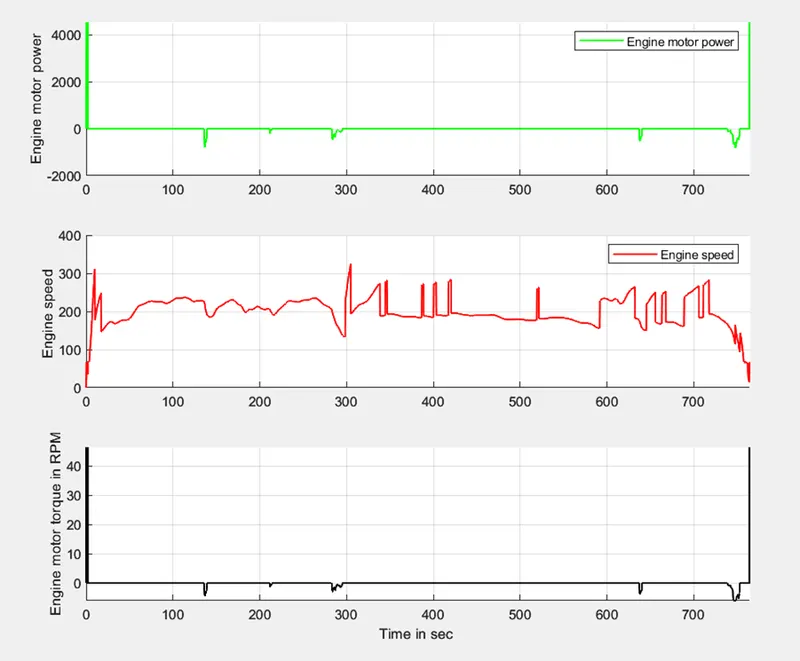
- Plot motor speed, torque, and motor input power using subplots.
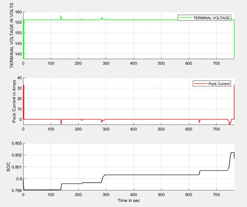
- Plot pack voltage, current, and SoC using subplots.
- Plot the motor operating points on the motor input power map, with the motor max motoring and generating torque curves.
- Write down appropriate brief comments on each plot, describing the vehicle behavior throughout the drive cycle.
- Generate the plots for both drive cycles
STUDY
The P1 architecture, with the electric machine connected directly to the crankshaft, is the solution adopted by Honda on their first generation Integrated Motor Assist (IMA) technology. The electric motor functions as a generator, during vehicle deceleration, as an engine starter, and as a motor (to assist the engine) during vehicle accelerations.
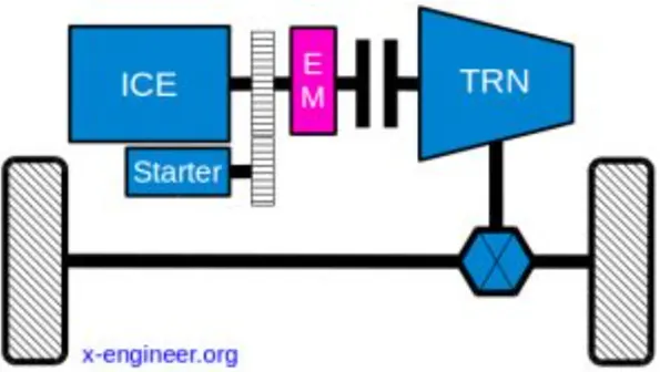
One of the biggest advantages of this solution is that the electric motor can provide higher torque than the BiSG, since there is no belt limitation (due to slip). However, since there is no speed/torque ratio between the electric machine and the crankshaft, the torque requirements on the electric motor can be quite demanding.
The primary advantage of a P1 mild hybrid architecture, compared with P0, is the removal of the belt drive. This means that the efficiency increases a bit (no more belt losses) and the electric machine torque can be higher in terms of amplitude and response (no more belt slip).
The functions (modes) performed by this mild hybrid topology are similar to those of a BiSG (P0), but, overall, P1 configurations have two big disadvantages: higher cost and higher impact on the existing vehicle architecture. Therefore, vehicle manufacturers and system suppliers are not investing in the further development of crankshaft-mounted integrated starter generator solutions for MHEV applications.
Two examples of P1 MHEV architectures are:
- Honda Insight Hybrid 2009 (with Integrated Motor Assist technology)
- Mercedes Benz S400 Bluehybrid 2010
INTRODUCTION
- In the forward scheme, a driver model controls the vehicle in an attempt to follow the input driving cycle, and the vehicle speed is intrinsically a dynamic state.
- A driver controller is required to control the vehicle to follow the desired speed and set the start of the calculations. The controller is implemented to model the driver that will either push the accelerator or the brake pedal to match the desired speed which enables to study of the driver's behavior. The controller is used as part of a feedback loop that will determine the energy required to drive the vehicle.
- Analytical models are representative of the Vehicle behavior and can be developed in MATLAB/Simulink by creating a vehicle model. They are based on fundamental theoretical equations. A model of the vehicle dynamics is built based on vehicle dynamics theory to calculate the power required at the wheels to overcome the resistance forces opposed to the vehicle motion: Aerodynamic Drag, Rolling, Inertia, Gradient, and Transmission resistances. The power required derives from the tractive force expressed as the sum of the resistances forces above
- The Simulink model for the convection model is created using 3 main subblocks for the driver model, the control model, and the powertrain block.
Vehicle Model
The vehicle model has to be designed in a MatLab environment. before we go into the designing side, we have to consider some basic parameters which come into the vehicle model design. We need to consider the vehicle parameters, road characteristics, Drive cycles, etc. So we build a Matlab script that loads all these variables and calculates some parameters which make a basic vehicle model.
Initialization File :
%%%%%%%%%%%%%%%%%%%%%%%%%%%%%%%%%%%%%%%%%%%%%%%%%%%%%%%%%%%%%%%%%%%%%
%% Skill-Lync -> Hybrid Drives Development
% Project 1 - Conventional Vehicle Model
% By - Arjundev
% Description:
%% Initialization File
% Initialization file for loading the variables for the Conventional vehicle simulation model
%% Vehicle Parameters
M = 1500; % Vehicle weight [kg]
Cr = 0.015; % Rolling resistance coefficient
Rw = 0.35; % Rolling radius [m]
Cd = 0.33; % Drag coefficient
Af = 2; % Frontal area [m2]
rhoa = 1.225; % Air density [kg/m3]
Vwind = 0; % Wind velocity [kmph]
g = 9.81; % Gravitational acceleration [m/s2]
theta = 0; % Slope [deg]
myu_road_tire = 1; % Coefficient of friction between tire - road interface
%% Powertrain Parameters
FDR = 3.73; % Final Drive Ratio / Diff Ratio
DiffEff = 0.99; % Differential efficiency (assumed independent of operating conditions)
NumGear = 4; % Number of gears in transmission
TransGear = [1:NumGear]; % Transmission Gears
TransRatio = [3.06, 1.62, 1, 0.7]; % Corresponding Transmission ratios
TransEff = 0.90; % Transmission efficiency (assumed independent of operating conditions)
TC_SR = [0, .5, .6, .7, .8, .87, .92, .94, .96, .97, 1]; % Torque Converter Speed Ratio (Matlab default) -> TurbSpd/PumpSpd
TC_TR = [2.232, 1.5462, 1.4058, 1.2746, 1.1528, 1.0732, 1.0192, 1, 1, 1, 1]; % Torque Converter Torque Ratio (Matlab default) -> TurbTrq/PumpTrq
TC_Cf = 1e-4 * [.72558, .66322, .63463, .59042, .51331, .4144, .29287, .22444, .12186, .04386, 0]; % Torque Converter Capacity Factor (Matlab default) -> PumpTrq/PumpSpd^2 [Nm/rpm^2]
load Vehicle_Data/Engine_data_1_9L_Saturn_95kW
load Vehicle_Data/Trans_Shift_map
load Vehicle_Data/EM_Honda_Insight_10kW
load Vehicle_Data/ESS_NiMH6
ESS_init_soc = 0.8;
ESS_soc_max = 0.9;
ESS_soc_min = 0.6;
%% Driver Parameters
Kp = 10; % P gain for driver PI model
Ki = 1; % I gain for driver PI model
Drive_Cycle_Select = 2; % Drive cycle selection
% Drive cycle values in m/s
if Drive_Cycle_Select == 1
load DriveCycles/UDDS;
elseif Drive_Cycle_Select == 2
load DriveCycles/HWFET;
elseif Drive_Cycle_Select == 3
load DriveCycles/FTP;
elseif Drive_Cycle_Select == 4
load DriveCycles/US06;
elseif Drive_Cycle_Select == 5
load DriveCycles/NEDC;
elseif Drive_Cycle_Select == 6
load DriveCycles/WLTP;
end
time_end = cyc_time(end);
vel_end = cyc_vel(end);
%%%%%%%%%%%%%%%%%%%%%%%%%%%%%%%%%%%%%%%%%%%%%%%%%%%%
Vehicle Model
The Simulink environment is used to create the basic vehicle model for a p1 hybrid electric vehicle. The parameters are preloaded in the Matlab environment and the parameters are taken into the Simulink environment.
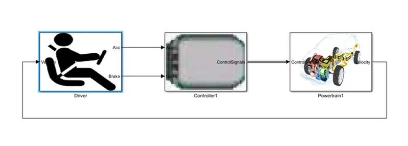
A basic vehicle model contains 3 major subsystems. They are given below.
- The driver system
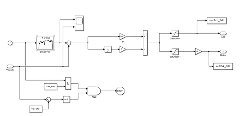
A basic driver system takes the drive cycle input from the Matlab environment and converts it into acceleration and brake pedal commands.
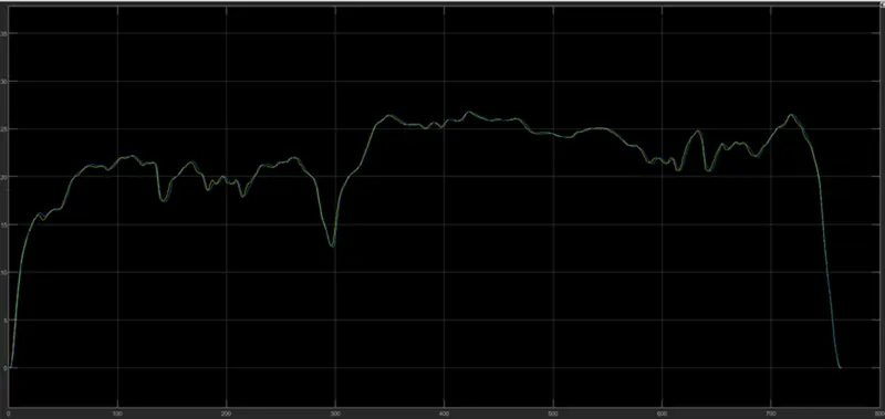
We can see there is an actual feedback system connected to the vehicle subsystem which gives us the actual velocity of the vehicle. this is further compared with the desired vehicle velocity and using the PI controller the errors are narrowed down. A comparison of desired and actual velocity plots is given below.
- Control system
The control system converts the acceleration and brake pedal inputs to required vehicle parameter requirements.
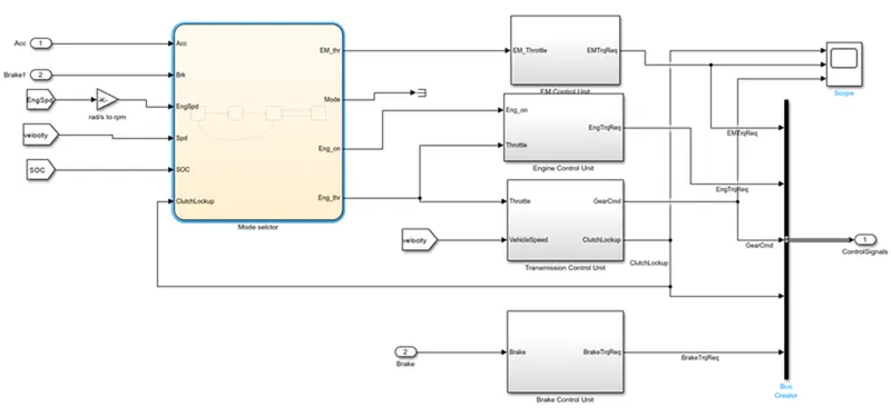
Inside this control system, there are 4 subsystems that control different vehicle systems as per the decision from the mode selector. Based on the driver inputs the controller generates desired engine torque, desired transmission gear, and desired brake torque.
The Mode selector :
The mode selector is a state flow chart from Simulink and can be considered as the brain of the whole vehicle system. this module selects the gear and decides when the electric motor or engine needs to be switched on and how much throttle needs to be transferred to which motor.
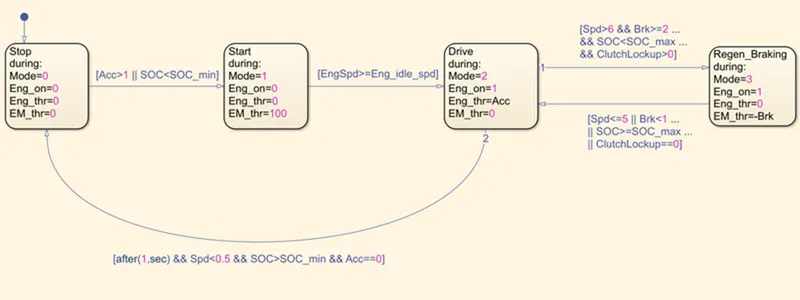
The Input to the state flow charts is Acceleration and Brake pedal input from the driver unit, Engine's actual
speed, Actual vehicle speed, SOC status, and the clutch lockup state. And the State flow Outputs to the
individual controllers are the Mode, Engine On/ off request, Engine input throttle, and Electric motor input Throttle
The controller consists of an engine control unit, a transmission control unit, an Electric Motor control unit, and a brake control unit. and they are given below.
The Electric motor control unit
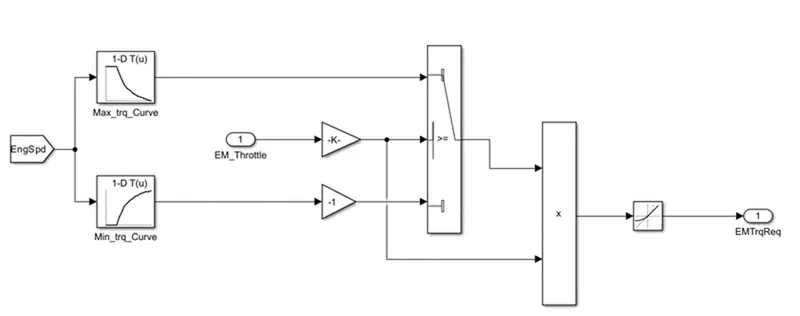
This controller converts the electric motor throttle demand which is coming from the mode selector to the torque requirement from the mode selector and is fed into the electric motor.
The Engine control Unit
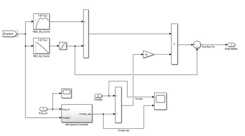
This controller converts the engine throttle demand which is coming from the mode selector to the torque requirement from the mode selector and is fed into the engine.
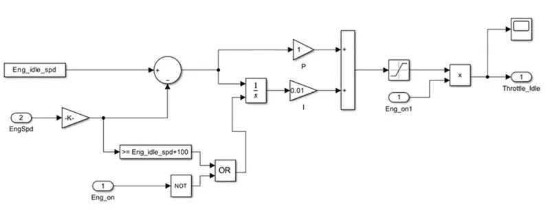
The idle speed controller
The Transmission control unit.
The transmission control unit takes the command of throttle and clutch lockup and decides which gear needs to be selected for the required speed of the vehicle. in order to achieve maximum efficiency for a particular gear the clutch has to be locked up so that the pump and turbine run at the same speed, this is decided and the required control is fed from this particular control unit.
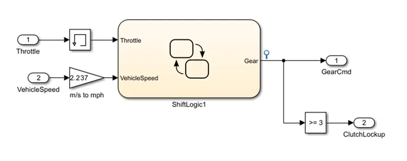
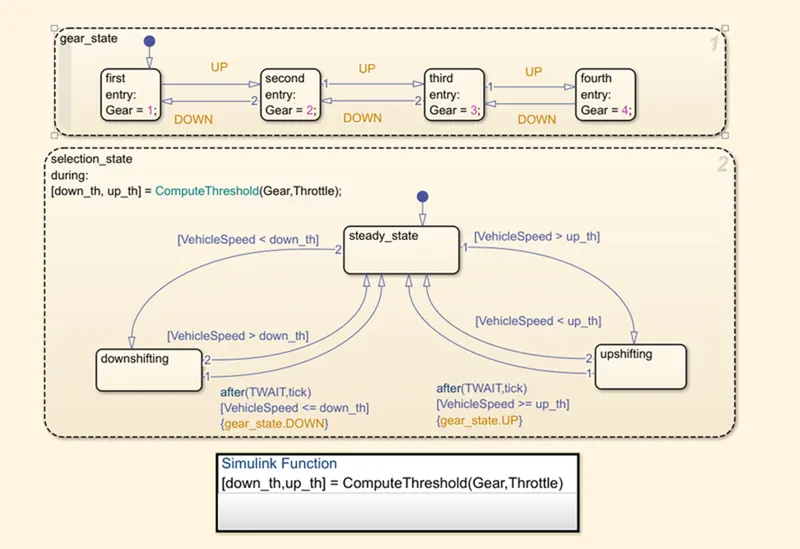
The shift logic.
The brake control unit
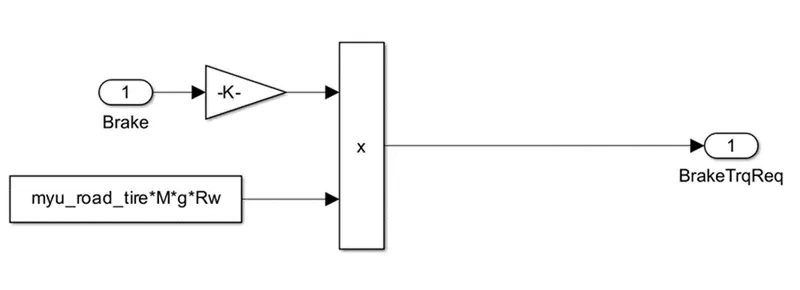
The Brake Control unit Produces the required brake torque according to the brake pedal input and passes the brake torque into the wheel block in the transmission model.
POWERTRAIN MODEL
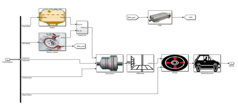
The powertrain model takes the controls from the control unit and performs the desired operations to get the desired vehicle velocity. It has 7 subsystems that are Electric motor, battery system, Engine, Transmission, Differential, Wheels, and Vehicle Dynamics. In the crank hub, the addition of both torques which are created by the engine and electric motor.
The Engine model.
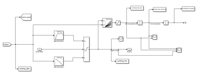
The Engine mode is a map-based model in which the engine speed is compared with the speed-torque curves as per the required demand torque and is considered and fed into the crank hub as engine torque. The 2D lookup table takes engine speed and generated torque and gives the fuel consumption rate and is further integrated to get fuel consumption and distance traveled. These quantities are passed on to the Matlab environment using to workspace tab.
The Electric motor model.
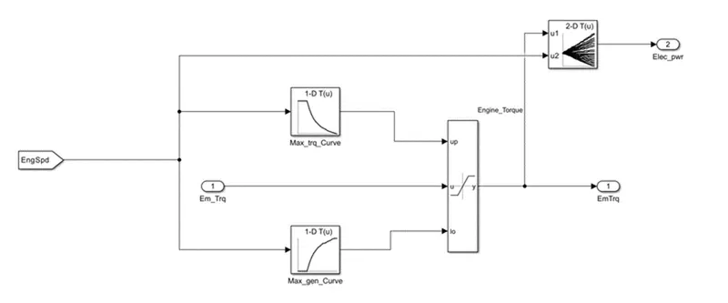
The Electric control unit is another map-based model which has an input of engine speed as this is a P1 model, and compares with the torque requirement from the control unit and gives the electric motor torque generated. The 2D lookup table gives the energy requirement and is fed into the battery system.
The Battery system:
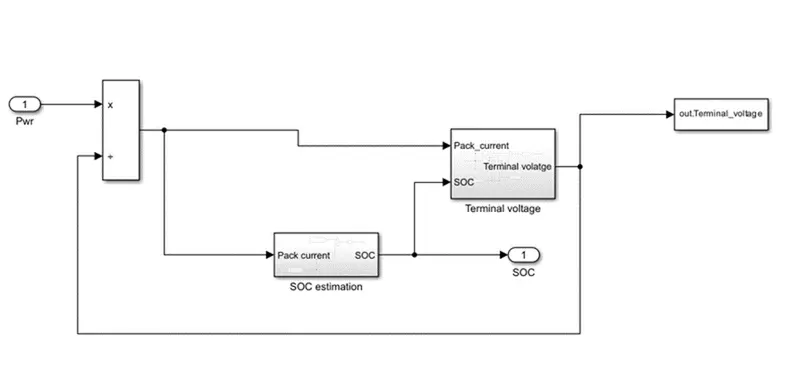
The battery subsystem takes in electric power requirement from the E-motor and gives output as SOC which is fed back to the mode selector.
The battery pack consists of two major subsystems and they are SOC estimation and terminal voltage.
The SOC Estimation
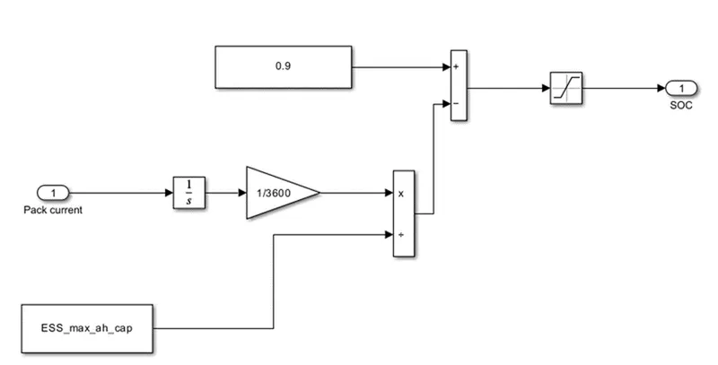
Pack current in Ampere is converted to AmpHour and divides with Max Capacity and adds with the Initial soc
to determine the SOC of the battery at each instance, the SOC value is limited between 0 to 1.
The Terminal voltage model
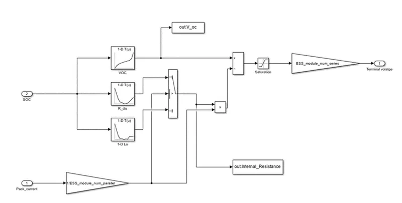
The model uses a 1D lookup table to estimate the pack's ideal voltage and internal resistance and determines the terminal voltage, and is fed back to the workspace for further study.
The Transmission model.
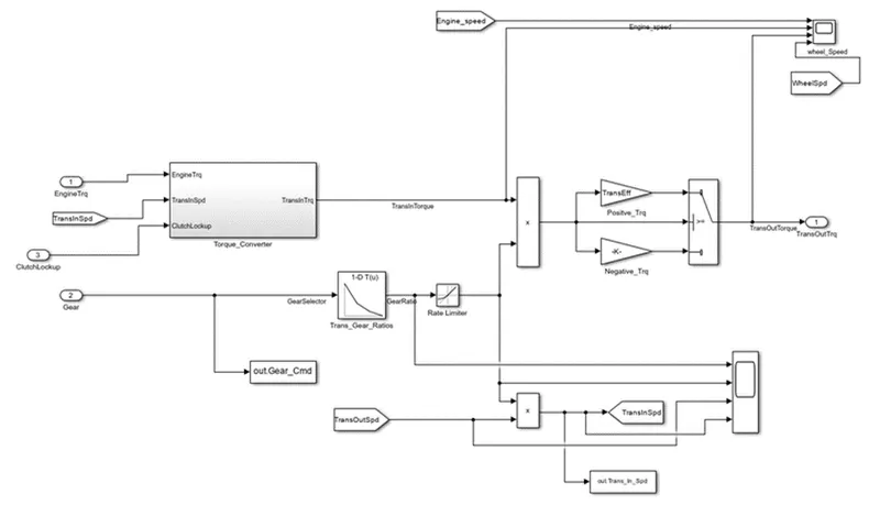
In these models, we take engine torque, and gear selector from the controller for transmission of gear ratio. The ratio is multiplied by the transmission input torque and then the transmission efficiency positive torque and negative torque give the transmission input speed. In this case, the torque converter connects the engine to the transmission it is part of the transmission. In it basically, engine dynamics are decoupled.
The Torque converter
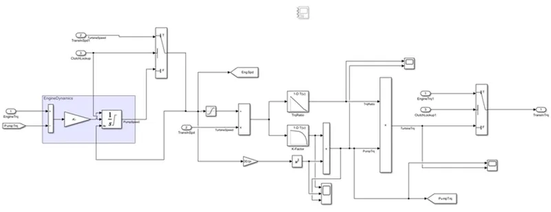
The Torque converter considers the turbine and pump torques and levels them to give the required torque output.
The crank hub
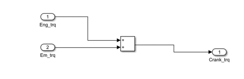
The crank hub adds the EM torque and the Engine torque to give a combined torque for transmission.
Differential Model
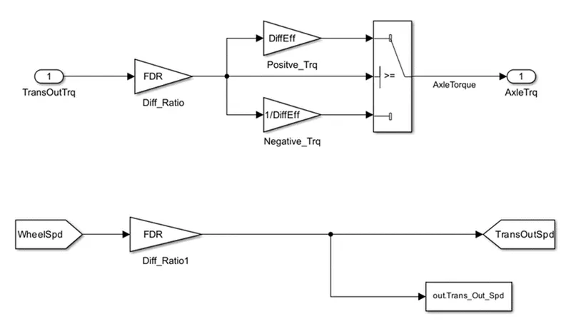
In the differential model, the input is the transmission output then it's going to the differential ratio multiplied by the output and input torque then meet axle torque. The axle torque is lower than the transmission torque and differential ratio.
Wheels:
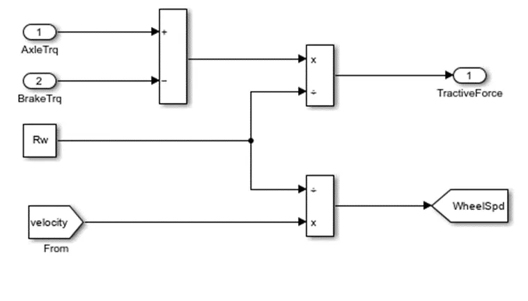
In this model, we take the axle torque from the differential and the brake torque from the controller. it is subtracting and multiplying rolling radius and velocity then we meet the tractive force from the axle and brake torque. and the wheel speed is met using velocity.
The Vehicle Model
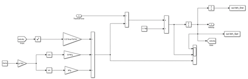
The vehicle subsystem is a mathematical model which is constructed under the relationship of tractive force with acceleration force, aerodynamic drag, and rolling resistance.
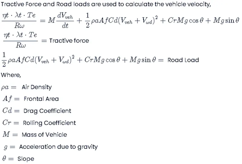
Then we calculate and integrate then we meet the acceleration of the vehicle and velocity of the vehicle which means vehicle distance and vehicle speed.
The Processing file
%%%%%%%%%%%%%%%%%%%%%%%%%%%%%%%%%%%%%%%%%%%%%%%%%%%%%%%%%%%%%%%%%%%%%
%% Skill-Lync -> Hybrid Drives Development
% Project 1 - Conventional Vehicle Model
% By - ARJUNDEV V V
% Description:
% The following file is to used with the Initialization file and Simulink
% results for post-processing of the data.
% The file is incomplete, has some examples of how the data is imported
% into a readable format, data analysis and plotting examples.
% Based on the project task, use commands in a similar format as given
% below, to analyse the data and generate required plots.
% You can change variable names if desired
%% Post-Processing File
% File for post-processing the Conventional vehicle simulation model data
%% Renaming variables
Time = out.tout;
Acc_Pdl = out.Acc_Pdl; % Accelerator pedal [%]
Brk_Pdl = out.Brk_Pdl; % Brake pedal [%]
Gear_Cmd = out.Gear_Cmd; % Transmission gear
Trans_In_Spd = out.Trans_In_Spd*30/pi; % Transmission input speed [rpm]
Trans_Out_Spd = out.Trans_Out_Spd*30/pi;% Transmission output speed [rpm]
Eng_Trq = out.Eng_Trq; % Engine brake torque [Nm]
Eng_Spd = out.Eng_Spd*30/pi; % Engine speed [rpm]
Eng_Fuel_Consump = out.Eng_Fuel_Consump; % Engine fuel consumption [g]
Veh_Dist = out.Veh_Dist/1000; % Distance traveled by vehicle [km]
Veh_Spd = out.Veh_Spd*18/5; % Vehicle speed [kmph]
Wheel_Speed = out.WheelSpeed; % Wheel speed [kmph]
Eng_Fuel_Rate = out.Eng_Fuel_rate; % Engine fuel rate [%]
term_volt = out.term_volt; %Battery voltage in volts
Pack_Current = out.Pack_Current; %pack current in amps
SOC = out.SOC ; % battery state of charge
EMPwr= out.EMPwr ; %Engine power in watts
EMSpd = out.EMSpd ; %Engine motor speed
EMTrq = out.EMTrq ; %Engine motor torque
%% Data Analysis
Eng_Pwr = (Eng_Spd.*pi./30).*Eng_Trq./1000; % Engine brake power [kW]
rho_petrol = 0.7197; % Density of petrol [kg/L]
kmpl = Veh_Dist(end)/(Eng_Fuel_Consump(end)/1000/rho_petrol); % Fuel economy [kmpl]
%% Plotting vehicle characteristics time trace
figure(1)
subplot(4,1,1)
hold on
grid on
plot(Time, Acc_Pdl, 'linewidth', 1, 'Color', 'black');
plot(Time, Brk_Pdl, 'linewidth', 1, 'Color', 'red');
ylabel('Pedal [%]')
xlim([0, Time(end)]);
legend('Accel','Brake');
subplot(4,1,2)
hold on
grid on
plot(Time, Veh_Spd, 'linewidth', 1, 'Color', 'red');
ylabel('Speed [rpm]')
xlim([0, Time(end)]);
legend('Actual Vehicle speed');
subplot(4,1,3)
hold on
grid on
plot(Time, Gear_Cmd, 'linewidth', 1, 'Color', 'black');
xlim([0, Time(end)]);
xlabel('Time [s]');
ylabel('Gear');
subplot(4,1,4)
hold on
grid on
plot(Time,Veh_Dist , 'linewidth', 1, 'Color', 'black');
xlim([0, Time(end)]);
xlabel('Time [s]');
ylabel('Vehicle_distance');
%% Plotting engine operating points on engine fuel map
figure('Name','Engine Operating Points');
hold on
grid on
title('Engine Operating Points','fontsize',12);
p1=plot(Eng_map_spd*30/pi,Eng_max_trq,'linewidth',2,'color','r');
p2=line([Eng_map_spd(end)*30/pi Eng_map_spd(end)*30/pi],[0 Eng_max_trq(end)]);
set(p2,'linewidth',1,'linestyle','--','color','k');
p3=line([Eng_map_spd(1)*30/pi Eng_map_spd(1)*30/pi],[0 Eng_max_trq(1)]);
set(p3,'linewidth',1,'linestyle','--','color','k');
[c,h] = contour(Eng_map_spd'*30/pi,Eng_map_trq,Eng_fuel_map');
clabel(c,h);
xlabel('Engine Speed [rpm]');
ylabel('Engine Torque [Nm]');
title('Engine Fuel Consumption Map [g/s]');
p4 = plot(Eng_Spd,Eng_Trq,'--','color','k');
legend([p1 p4],{'Max Curve','Operating Points'});
axis([Eng_map_spd(1)*30/pi Eng_map_spd(end)*30/pi 0 Eng_map_trq(end)]);
figure(3)
subplot(4,1,1)
hold on
grid on
plot(Time, Eng_Spd, 'linewidth', 1, 'Color', 'Green');
ylabel('Engine speed in Km/h')
xlim([0, Time(end)]);
legend('Engine speed');
subplot(4,1,2)
hold on
grid on
plot(Time, Eng_Pwr, 'linewidth', 1, 'Color', 'red');
ylabel('Engine Power in W')
xlim([0, Time(end)]);
legend('Engine Power');
subplot(4,1,3)
hold on
grid on
plot(Time, Eng_Fuel_Rate, 'linewidth', 1, 'Color', 'black');
xlim([0, Time(end)]);
xlabel('Time [s]');
ylabel('Engine fuel rate');
subplot(4,1,4)
hold on
grid on
plot(Time,Eng_Fuel_Consump , 'linewidth', 1, 'Color', 'black');
xlim([0, Time(end)]);
xlabel('Time [s]');
ylabel('Engine fuel consumption');
figure('Name','Engine Operating Points');
hold on
grid on
title('Electric motor Operating Points','fontsize',12);
p1=plot(EM_map_spd*30/pi,EM_max_trq,'linewidth',2,'color','r');
p2=line([(EM_map_spd(end)).*30/pi (EM_map_spd(end)).*30/pi],[0 EM_max_trq(end)]);
set(p2,'linewidth',1,'linestyle','--','color','k');
p3=line([EM_map_spd(1)*30/pi EM_map_spd(1)*30/pi],[0 EM_max_trq(1)]);
set(p3,'linewidth',1,'linestyle','--','color','k');
[c,h] = contour(EM_map_spd'*30/pi,EM_map_trq,EM_inpwr_map');
clabel(c,h);
xlabel('E-Motor Speed [rpm]');
ylabel('E-Motor Torque [Nm]');
title('E-Motor Power Map [g/s]');
p4 = plot(Eng_Spd,Eng_Trq,'--','color','k');
legend([p1 p4],{'Max Curve','Operating Points'});
axis([EM_map_spd(1)*30/pi EM_map_spd(end)*30/pi 0 EM_map_trq(end)]);
figure(7)
subplot(3,1,1)
hold on
grid on
plot(Time, EMPwr, 'linewidth', 1, 'Color', 'Green');
ylabel('Engine motor power')
xlim([0, Time(end)]);
legend('Engine motor power');
subplot(3,1,2)
hold on
grid on
plot(Time, EMSpd, 'linewidth', 1, 'Color', 'red');
ylabel('Engine speed ')
xlim([0, Time(end)]);
legend('Engine speed');
subplot(3,1,3)
hold on
grid on
plot(Time, EMTrq, 'linewidth', 1, 'Color', 'black');
xlim([0, Time(end)]);
xlabel('Engine motor torque in RPM ');
ylabel('Engine motor');
figure(6)
subplot(3,1,1)
hold on
grid on
plot(Time, term_volt, 'linewidth', 1, 'Color', 'Green');
ylabel('TERMINAL VOLTAGE IN VOLTS')
xlim([0, Time(end)]);
legend('TERMINAL VOLTAGE');
subplot(3,1,2)
hold on
grid on
plot(Time, Pack_Current, 'linewidth', 1, 'Color', 'red');
ylabel('Pack Current in Amps')
xlim([0, Time(end)]);
legend('Pack Current');
subplot(3,1,3)
hold on
grid on
plot(Time, SOC, 'linewidth', 1, 'Color', 'black');
xlim([0, Time(end)]);
xlabel('SOC in %');
ylabel('SOC');
THE PLOTS AND RESULT.
1.the fuel economy numbers (kmpl) for UDDS and HWFET cycle
The Fuel economy for HWFET is 17.1565
The Fuel economy for UDDS is 14.7541
As compared to both the driving demands the highway drive gives us better fuel efficiency than Urban drive due to frequent change speed and torque demand and project 2 fuel economy is bit higher when compared to project 1 as the electric motor assistance by P1 architecture.
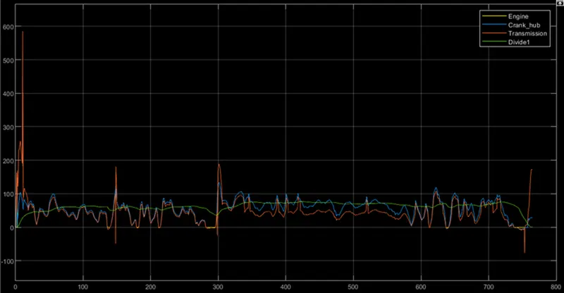
- Time trace for engine, transmission input, transmission output, and wheel speed on one plot.
For HWFET,
For UDDS,
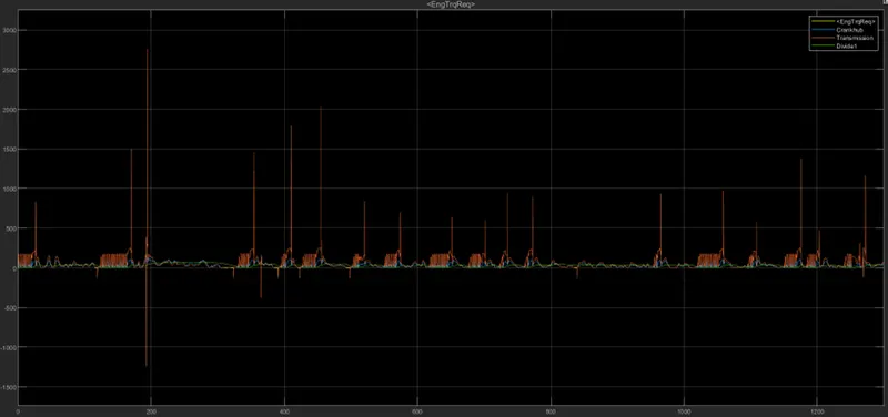
We can see that in UDDS the graph is fluctuating that HWFET as the traffic is more comparatively. And breaking is high for UDDS that HWFET
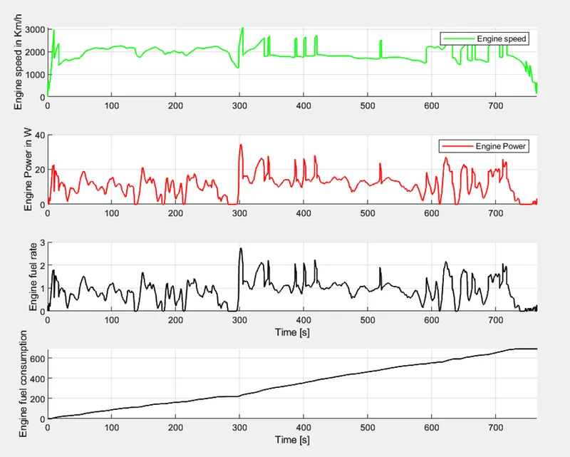
3. Engine torque, engine power, fuel rate, and fuel consumption
For HWFET
For UDDS,
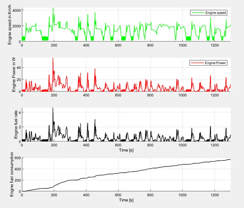
As we look into the engine speed for both drive cycles, UDDS is fluctuating more immediately than HWFET. The power consumption high for HWFET than UDDS and the fluctuation is lesser. The fuel rate is high in the HWFET drive cycle compared to the UDDS drive cycle. The fuel rate is lower for UDDS when compared to HWFET. Fuel economy is lesser in UDDS as the frequent change in speed and start-stop affect fuel efficiency.
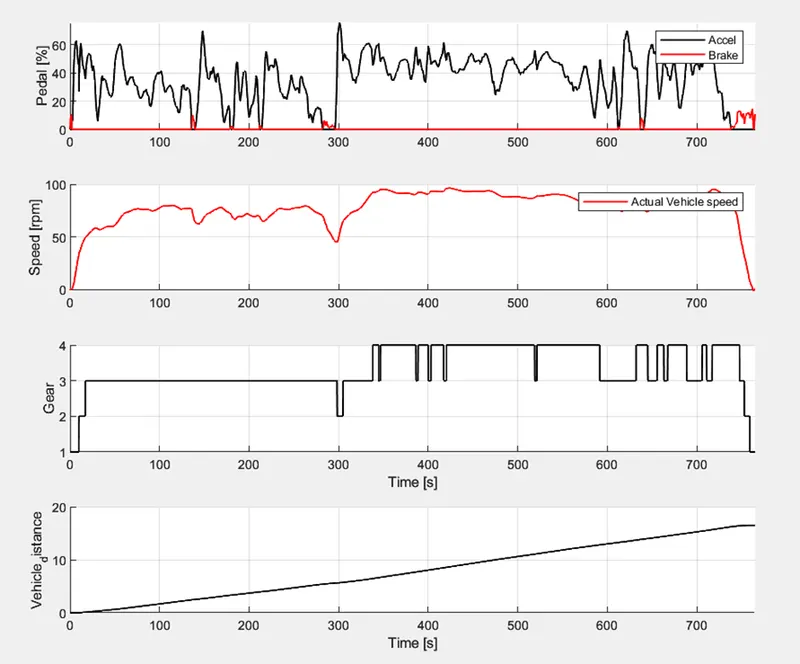
4. Accelerator and brake pedal, gear command, vehicle desired and actual speed, vehicle distance
For HWFET
For UDDS
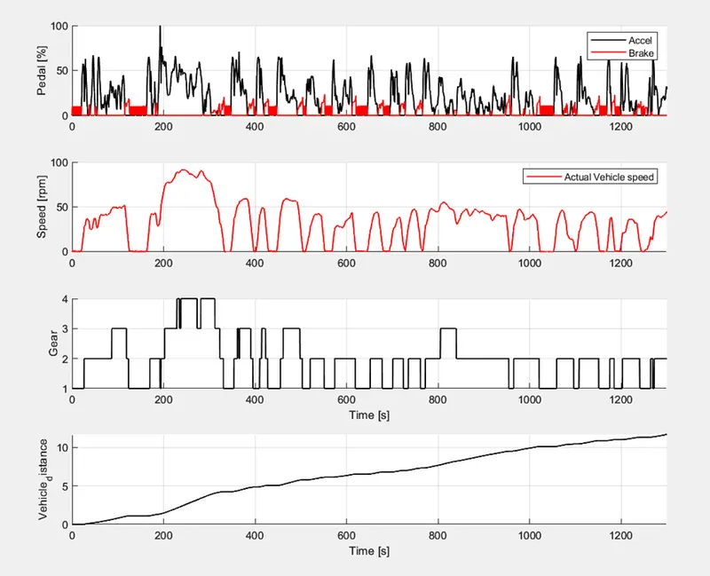
The pedal engagement is entirely different in both cycles as the start-stop operation in UDDS is clearly visible in this plot. The speed actually follows the normal drive cycle plots. and we can see that the gear engagement is also affected by this cycle selection, the HWFET cycle usually operates in the 3,4 gears whereas in UDDS the gears engage as per the pedal requirement and we can see more 1 and 2 gears.
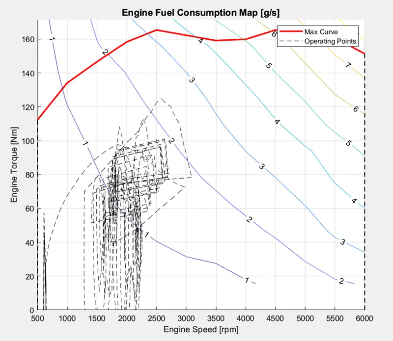
- Engine operating points on the engine fuel map
For HWFET
For UDDS,
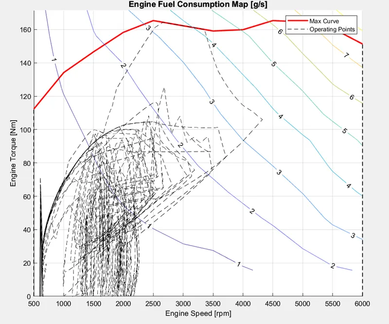
As we compare both plots we can see that there is a clear difference in the operating points of UDDS and HWFET cycles. The points are distributed in UDDS whereas in HWFET for a steady demand.
6.motor speed, torque, and motor input power using subplots.
For HWFET
For UDDS
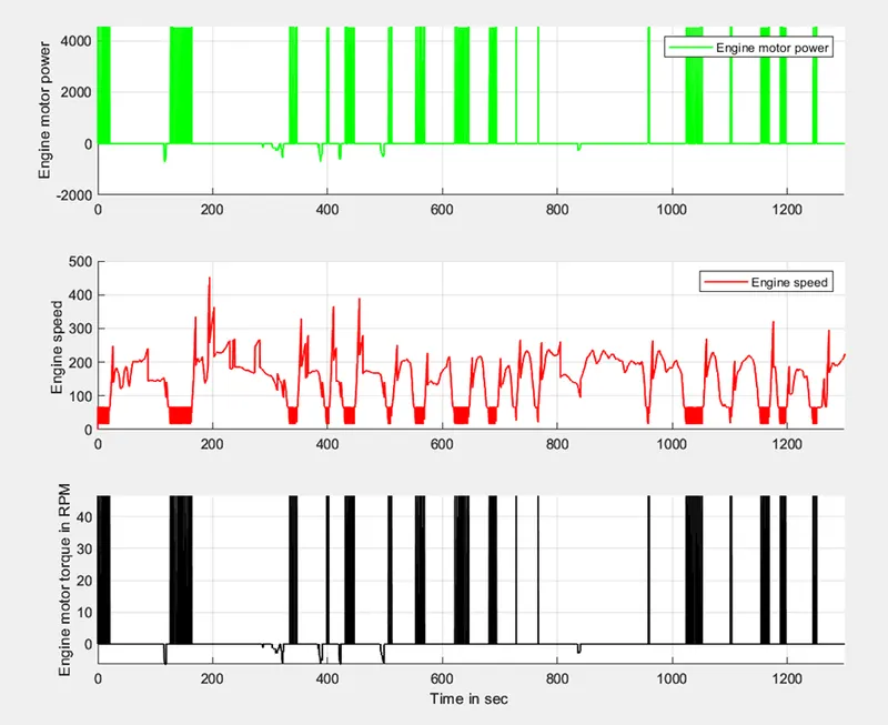
The Fluctuation is clearly visible in UDDS as the demand in the cycles compared to HWFET has the same plots.The HWFET has a smooth plot. We can observe that the motor power and torque are high in HWFET and in UDDS it has continued fluctuations this is because of frequent braking in UDDS
- pack voltage, current, and SoC using subplots.
For HWFET
For UDDS,
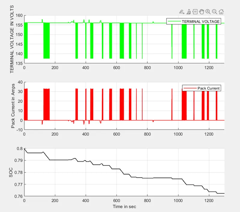
As per the motor speed torque and power plots, we get the same result here. The fluctuation is high for UDDS when compared to HWFET . The SOC is getting charged for HWFET whereas the alternate is simply charged due to smooth driving, in UDDS the demand and frequent start and stop deplete the SOC.
8. Motor operating points on the motor input power map, with the motor max motoring and generating torque curves.
For HWFET,
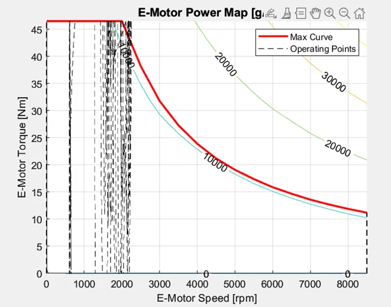
For UDDS,
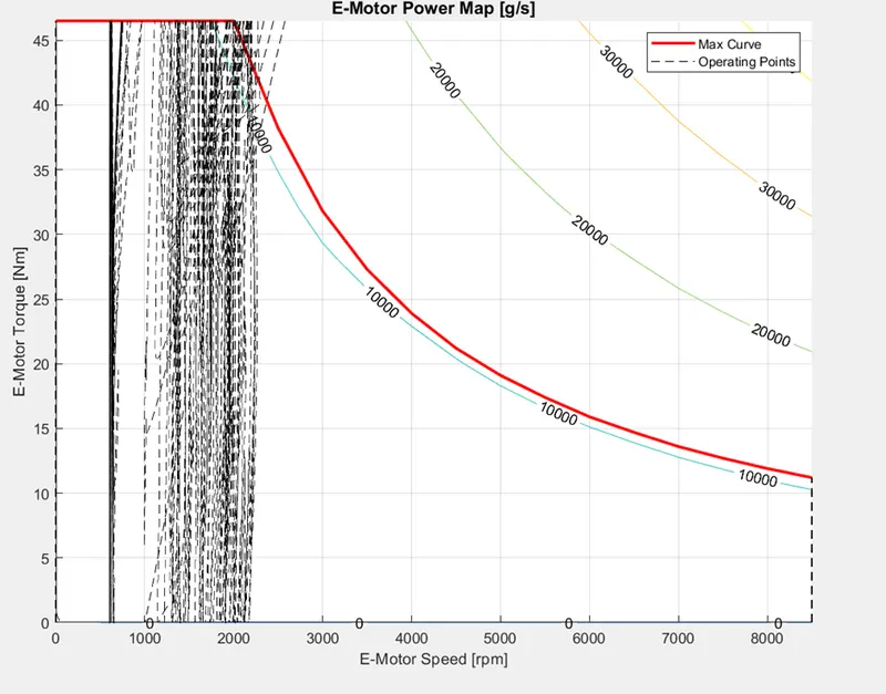
Conclusion.
We have developed a P1 hybrid powertrain model and evaluated it for both HWFET and UDDS drive cycles.
- The time trace for the engine, transmission input, transmission output, and wheel speed is Plotted and compared for both cycles
- The engine torque, engine power, fuel rate, and fuel consumption are Plotted and compared for both cycles
- The accelerator and brake pedal, gear command, vehicle desired and actual speed, and vehicle distance is Plotted and compared for both cycles
- the engine operating points on the engine fuel map are Plotted and compared for both cycles
- motor speed, torque, and motor input power are Plotted and compared for both cycles
- pack voltage, current, and SoC are Plotted and compared for both cycles
- the motor operating points on the motor input power map, with the motor max motoring and generating torque curves are Plotted and compared for both cycles
- We have also compared the Conventional and p1 hybrid fuel economy and studied that the P1 architecture gives us more fuel efficiency than conventional designs.