Project 2
P1 Hybrid Architecture:
Positioned between the engine and transmission, the P1 hybrid architecture and Integrated Starter Generator enable high-efficiency power generation while featuring regenerative braking and acceleration assist. This hybrid technology enables high-efficiency power generation and motoring capability in a highly flexible package designed to fit between the engine and transmission.
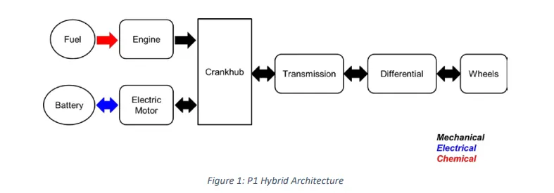
Honda Insight motor and battery are considered for this project. The details on the type of motor and battery are shown below.

Modeling P1 Hybrid Architecture in MatLab:
Initialization:
An Initialization file for loading the variables for the Hybrid vehicle simulation model has been created.
Simulink Model:
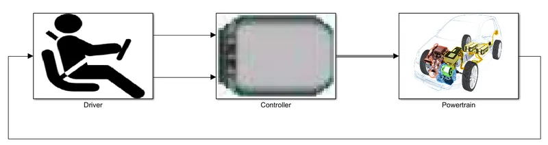
The plant model consists of a driver, controller, and a powertrain block.
DRIVER:
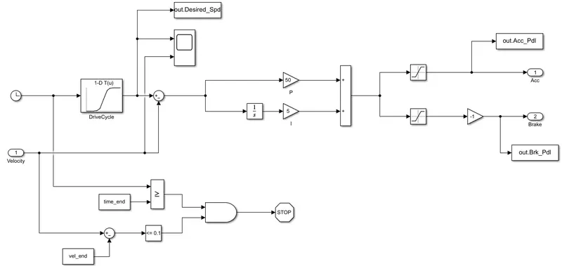
The Driver model block is a basic PI controller that generates accelerator and brake pedal outputs to match the desired and actual vehicle speeds. The PI controller minimizes the error between the required vehicle speed and the actual speed of the vehicle.
CONTROLLER:
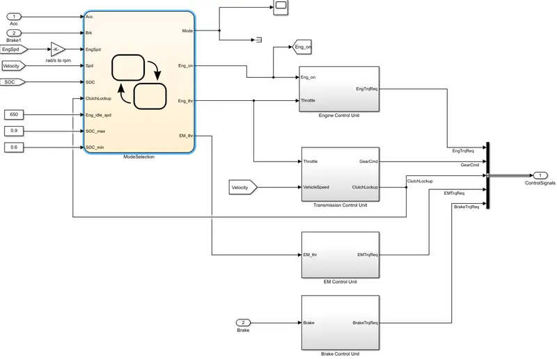
The controller block is the brain of the vehicle. It contains the ECU. Based on the driver inputs, the controller block generates the output and this is fed into the powertrain block of the system. The Controller block has a Mode Selection chart, created for the hybrid architecture, to choose the operating mode of the vehicle based on the driver inputs. Based upon this, the engine control unit, the transmission control unit, and the motor control unit generate output.
Engine Control Unit:
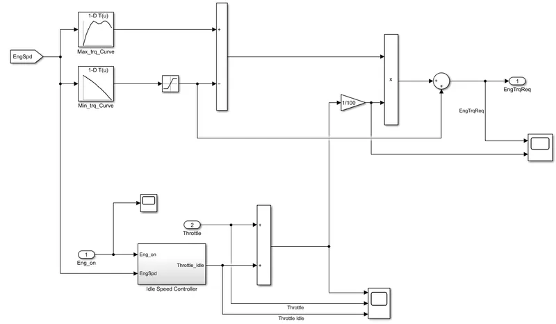
The engine control unit compares engine speed with the maximum torque and minimum torque curve of the lookup table and gives the required torque command to the engine block. An engine ON block was added to the idle throttle control so that the engine idling is 0 when it is off. The reason for adding it was to remove the excess fuel consumption of the engine during idling as the hybrid vehicle does not require the engine to be on during low speeds.
Transmission Control Unit:
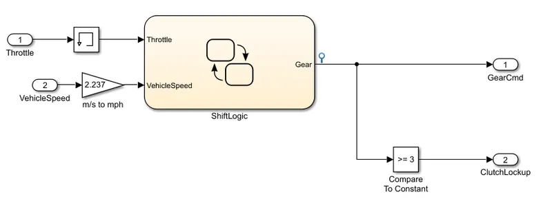
The transmission control block controls the gear shifting. The gear shifting is controlled according to the vehicle speed and throttle input.
Clutch lockup is added to generate output based on the conditions.
Electric Machine Control Unit:
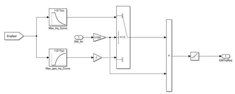
The EM control unit is similar to the engine control unit.
Brake Control Unit:
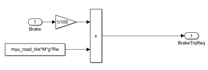
The brake control unit produces the required brake torque according to the brake pedal input.
POWERTRAIN:
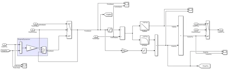
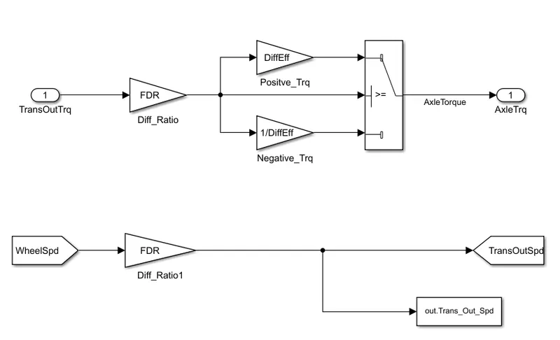
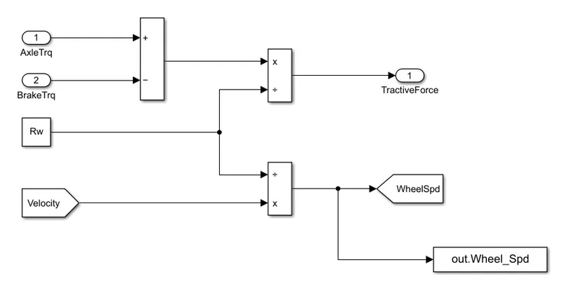
The Powertrain block represents the drivetrain of the vehicle. It consists of an Engine model along with an Electric Motor connected to the Automatic Transmission model through a Torque Converter. The output of the transmission is connected to the Differential, which powers the Wheels that provides the tractive force for vehicle acceleration. The longitudinal dynamics of the vehicle along with the road load are represented in the Vehicle Dynamics block.
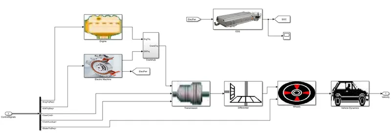
Engine:
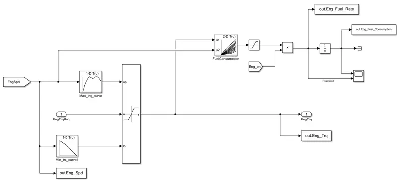
Electric Machine:
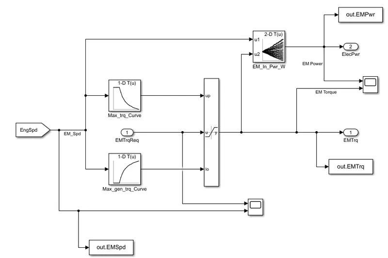
Crankhub:
The crank hub adds up the EM torque and the engine torque and passes it to the transmission block as the crank torque.
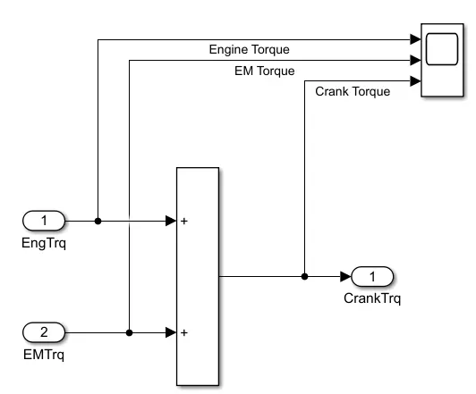
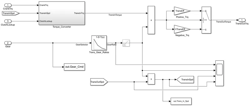
Transmission:
Torque Converter:
The clutch lockup input is fed into the torque converter block. It chooses between the pump speed and the turbine speed and calculates the Transmission Input speed.
Differential:
Wheels:
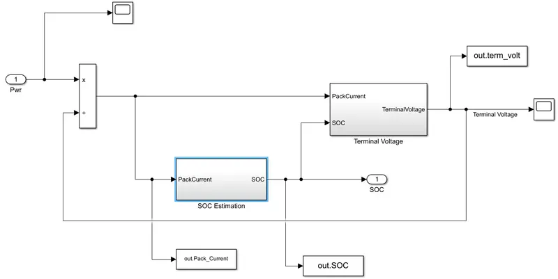
Energy Storage System:
The ESS is created with electric power input and battery SOC as output. The SOC is used to calculate the Terminal voltage.
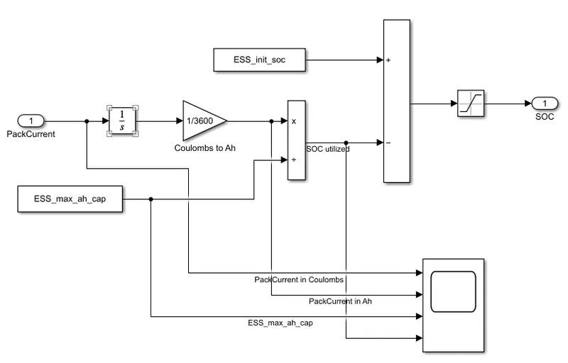
SOC:
The SOC is estimated based on the difference between the current SOC and the utilized SOC.
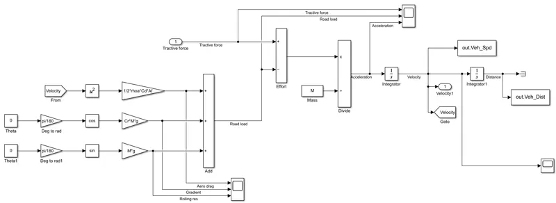
Vehicle Dynamics:
The longitudinal dynamics of the vehicle along with the road load is represented in the vehicle dynamics block. Tractive force and road loads are used to calculate the vehicle velocity.
MatLab Script for Post-Processing:
% Project 2 - Hybrid Vehicle Model
% File for post-processing the Hybrid vehicle simulation model data
%% Renaming variables
Time = out.tout;
Acc_Pdl = out.Acc_Pdl; % Accelerator pedal [%]
Brk_Pdl = out.Brk_Pdl; % Brake pedal [%]
Gear_Cmd = out.Gear_Cmd; % Transmission gear
Trans_In_Spd = out.Trans_In_Spd*30/pi; % Transmission input speed [rpm]
Trans_Out_Spd = out.Trans_Out_Spd*30/pi; % Transmission output speed [rpm]
Eng_Trq = out.Eng_Trq; % Engine brake torque [Nm]
Eng_Spd = out.Eng_Spd.*30/pi; % Engine speed [rpm]
Eng_Fuel_Consump = out.Eng_Fuel_Consumption; % Engine fuel consumption [g]
Eng_Fuel_Rate = out.Eng_Fuel_Rate; % Engine fuel rate [g]
Veh_Dist = out.Veh_Dist/1000; % Distance traveled by vehicle [km]
Veh_Spd = out.Veh_Spd*18/5; % Vehicle speed [kmph]
Wh_Spd = out.Wheel_Spd*30/pi; % Wheel speed [kmph]
Des_Spd = out.Desired_Spd*18/5; % Vehicle Desired speed [kmph]
EM_Spd = out.EMSpd.*30/pi; % Electric machine speed [rpm]
EM_Trq = out.EMTrq; % Electric machine torque [Nm]
EM_Pwr = out.EMPwr./1000; % Electric machine power [kW]
ESS_Pack_Volt = out.term_volt; % Battery pack voltage [V]
ESS_Pack_Cur = out.Pack_Current; % Battery pack current
SOC = out.SOC.*100; % Battery State of Charge
%% Data Analysis
Eng_Pwr = Eng_Spd.*pi/30.*Eng_Trq/1000; % Engine brake power [kW]
rho_petrol = 0.7197; % Density of petrol [kg/L]
kmpl = Veh_Dist(end)/(Eng_Fuel_Consump(end)/1000/rho_petrol); % Fuel economy [kmpl]
%% 1
% Plotting vehicle speed characteristics
figure(1)
hold on
grid on
plot(Time,Eng_Spd,'r',LineWidth=1);
plot(Time,Trans_In_Spd,'b',LineWidth=1);
plot(Time,Trans_Out_Spd,'k',LineWidth=1);
plot(Time,Wh_Spd,'g',LineWidth=1);
xlabel('Time [s]');
ylabel('Speed [kmph]');
title('Speed Vs Time');
xlim([0,Time(end)]);
legend('Engine Speed','Transmission Input Speed','Transmission Output Speed','Wheel Speed');
%% 2
% Plotting engine characteristics
figure(2)
subplot(4,1,1)
title('Engine Characteristics')
hold on
grid on
plot(Time,Eng_Trq,'b',LineWidth=1);
ylabel('Engine Torque [Nm]');
xlim([0,Time(end)]);
legend('Engine Torque');
subplot(4,1,2)
hold on
grid on
plot(Time,Eng_Pwr,'r',LineWidth=1);
ylabel('Engine Power [kW]');
xlim([0,Time(end)]);
legend('Engine Power');
subplot(4,1,3)
hold on
grid on
plot(Time,Eng_Fuel_Rate,'g',LineWidth=1);
ylabel('Fuel rate [g]');
xlim([0,Time(end)]);
legend('Engine Fuel Rate');
subplot(4,1,4)
hold on
grid on
plot(Time,Eng_Fuel_Consump,'m',LineWidth=1 );
ylabel('Fuel Consumption [g]');
xlabel('Time [s]');
legend('Engine Fuel Consumption');
xlim([0,Time(end)]);
%% 3
% Plotting vehicle characteristics time trace
figure(3)
subplot(4,1,1)
title('Vehicle Characteristics');
hold on
grid on
plot(Time, Acc_Pdl,'k',LineWidth=1);
plot(Time, Brk_Pdl,'r',LineWidth=1);
ylabel('Pedal [%]');
xlim([0, Time(end)]);
legend('Accelerator','Brake');
subplot(4,1,2)
hold on
grid on
plot(Time, Gear_Cmd,'m',LineWidth=1);
xlim([0, Time(end)]);
ylabel('Gear');
subplot(4,1,3)
hold on
grid on
plot(Time, Des_Spd,'r',LineWidth=1);
plot(Time, Veh_Spd,'y',LineWidth=1,LineStyle='-');
xlim([0, Time(end)]);
ylabel('Speed [kmph]');
legend('Desired Speed', 'Actual Speed');
subplot(4,1,4)
hold on
grid on
plot(Time, Veh_Dist,'g',LineWidth=1);
xlim([0, Time(end)]);
xlabel('Time [s]');
ylabel('Distance [km]');
%% 4
% Plotting engine operating points on engine fuel map
figure(4)
hold on
grid on
title('Engine Operating Points');
p1=plot(Eng_map_spd*30/pi,Eng_max_trq,linewidth=2,color='r');
p2=line([Eng_map_spd(end)*30/pi Eng_map_spd(end)*30/pi],[0 Eng_max_trq(end)]);
set(p2,linewidth=1,linestyle='--',color='k');
p3=line([Eng_map_spd(1)*30/pi Eng_map_spd(1)*30/pi],[0 Eng_max_trq(1)]);
set(p3,linewidth=1,linestyle='--',color='k');
[c,h] = contour(Eng_map_spd'*30/pi,Eng_map_trq,Eng_fuel_map');
clabel(c,h);
xlabel('Engine Speed [RPM]');
ylabel('Engine Torque [Nm]');
title('Engine Fuel Consumption Map [g/s]');
legend([p1 p2],{'Max Curve','Operating Points'});
axis([Eng_map_spd(1)*30/pi Eng_map_spd(end)*30/pi 0 Eng_map_trq(end)]);
%% 5
% Plotting motor characteristics
figure(5)
subplot(3,1,1)
title('Motor Characteristics');
hold on
grid on
plot(Time,EM_Spd,'g',linewidth=1);
ylabel('Motor Speed [RPM]');
xlim([0,Time(end)]);
legend('Motor Speed');
subplot(3,1,2)
hold on
grid on
plot(Time,EM_Trq,'m',linewidth=1);
ylabel('Motor Torque [Nm]');
xlim([0,Time(end)]);
legend('Motor Torque');
subplot(3,1,3)
hold on
grid on
plot(Time,EM_Pwr,'r',linewidth=1);
ylabel('Motor Power [kW]');
xlabel('Time [s]');
xlim([0,Time(end)]);
legend('Motor Power');
%% 6
% Plotting Battery characteristics
figure(6)
subplot(3,1,1)
title('Battery Characteristics');
hold on
grid on
plot(Time,ESS_Pack_Volt,'r',linewidth=1);
ylabel('Pack Voltage [V]');
xlim([0,Time(end)]);
legend('Pack Voltage');
subplot(3,1,2)
hold on
grid on
plot(Time,ESS_Pack_Cur,'b',linewidth=1);
ylabel('Pack Current');
xlim([0,Time(end)]);
legend('Pack Currrent');
subplot(3,1,3)
hold on
grid on
plot(Time,SOC,'g',linewidth=1);
ylabel('SOC %');
xlabel('Time [s]');
xlim([0,Time(end)]);
legend('SOC');
%% 7
% Plotting motor operating points
figure(7)
hold on
grid on
title('Motor Operating Points');
p1=plot(EM_map_spd*30/pi,EM_max_trq,linewidth=2,color='r');
p2=line([EM_map_spd(end)*30/pi EM_map_spd(end)*30/pi],[0 EM_max_trq(end)]);
set(p2,linewidth=1,linestyle='--',color='k');
p3=line([EM_map_spd(1)*30/pi EM_map_spd(1)*30/pi],[0 EM_max_trq(1)]);
set(p3,linewidth=1,linestyle='--',color='k');
p4=plot(EM_map_spd*30/pi,EM_max_gen_trq,linewidth=2,Color='b');
p2=line([EM_map_spd(end)*30/pi EM_map_spd(end)*30/pi],[0 EM_max_gen_trq(end)]);
set(p2,linewidth=1,linestyle='--',color='k');
p3=line([EM_map_spd(1)*30/pi EM_map_spd(1)*30/pi],[0 EM_max_gen_trq(1)]);
set(p3,linewidth=1,linestyle='--',color='k');
[c,h] = contour(EM_map_spd'*30/pi,EM_map_trq,EM_inpwr_map');
clabel(c,h);
xlabel('Motor Speed [RPM]');
ylabel('Motor Torque [Nm]');
%title('Engine Fuel Consumption Map [g/s]');
legend([p1 p4 p2],{'Max Torque Curve','Max Gen Torque','Operating Points'});
axis([EM_map_spd(1)*30/pi EM_map_spd(end)*30/pi -46.5 EM_map_trq(end)]);
Simulation Results:
1. The fuel economy numbers (kmpl) for UDDS and HWFET cycle:
|
Drive Cycles |
Fuel Economy [kmpl] |
|
|
Conventional |
Hybrid |
|
|
UDDS |
14.2044 |
13.9948 |
|
HWFET |
16.5010 |
17.1429 |
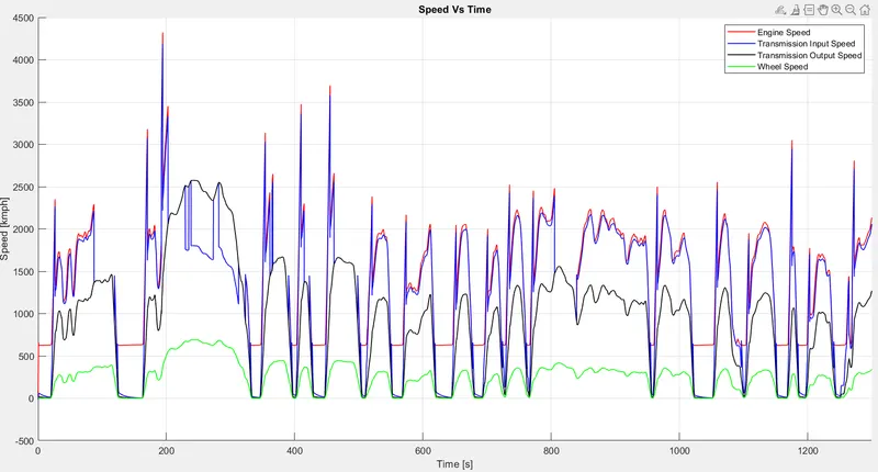
2. Vehicle Speed Characteristics
UDDS Cycle:
HWFET Cycle:
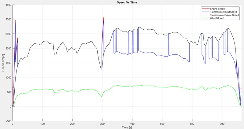
Observation: The Transmission input speed follows the engine speed but there are fluctuations due to the torque converter. The transmission output speed matches the engine speed on the 3rd and 4th gear i.e. overdrive and the wheel speed varies according to the gearing and final drive ratio.
3. Engine Characteristics
UDDS:
HWFET:
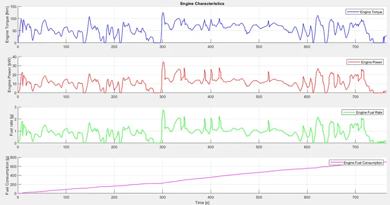
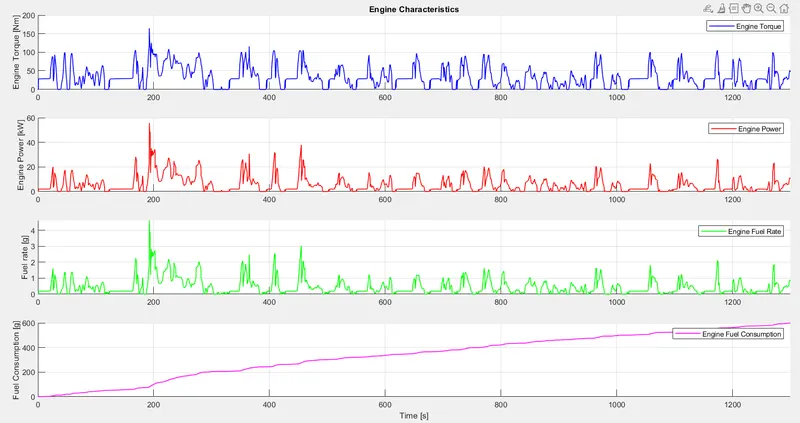
Observation: As the torque requirements are different according to the drive cycle, the fuel rate varies based on which the fuel consumption is calculated. The torque and power requirements are low on the UDDS cycle as it is operated in city traffic conditions. As for HWFET, the torque and power requirements are higher as it is driven on a highway.
4. Vehicle Characteristics
UDDS: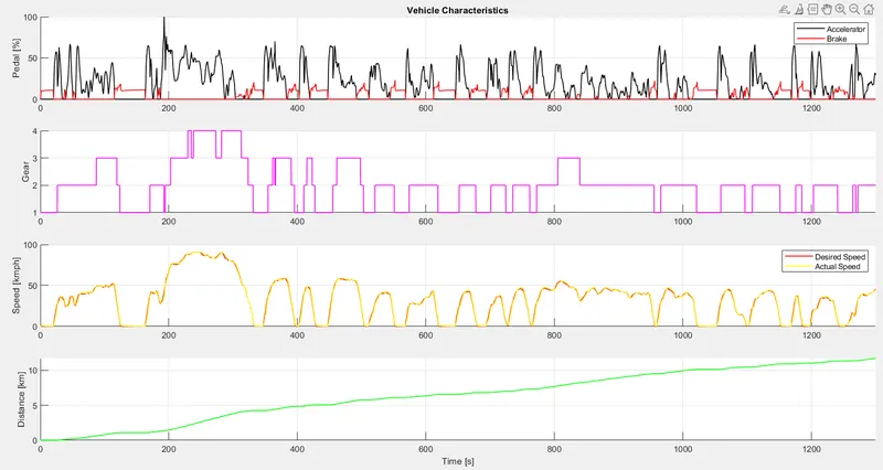
HWFET:
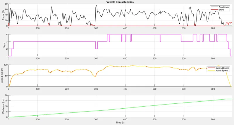
Observation: The UDDS cycle has many stops-and-go situations leading to multiple gear shifts and also more regen recovery is possible. In the case of HWFET, the brakes are not used that often and the gear shifts are also fewer. As for regen, it is less on the HWFET cycle.
5. Engine Operating Points
UDDS:
HWFET:
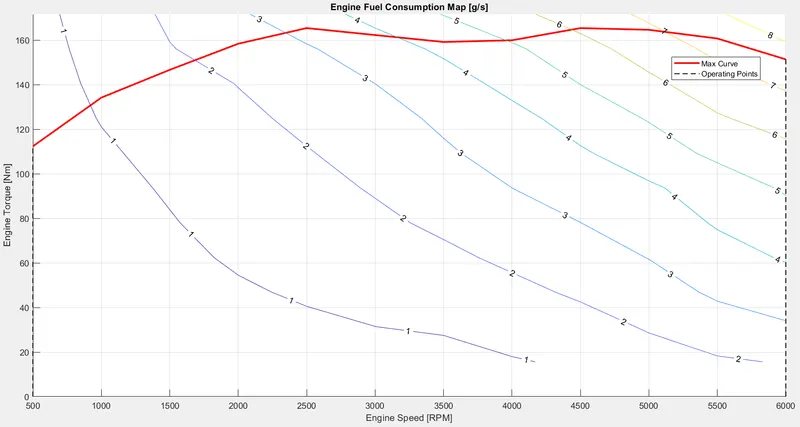
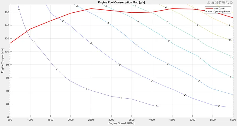
Observation: The engine operating points are well within the maximum torque curve for both cycles.
6. Motor Characteristics
UDDS: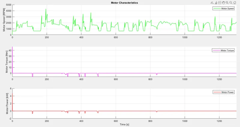
HWFET:
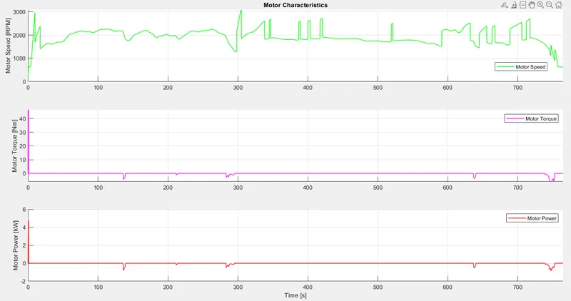
Observation: The motor torque is pretty much needed at the start of the vehicle and it is reflected in both cycles. The regen torque is mostly observed in the UDDS cycle as the usage of brakes is more.
7. Battery Characteristics
UDDS:
HWFET:
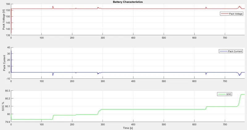
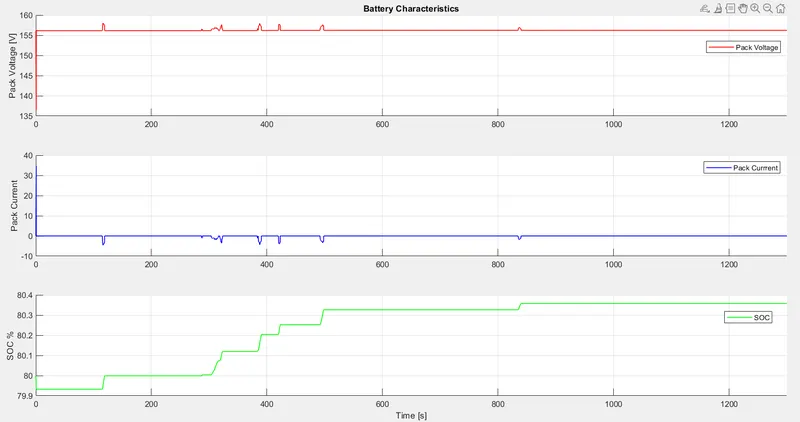
Observation: At the initial stage more current is consumed as the motor tries to start the engine. The battery is charged quite fast in the UDDS cycle as compared to the HWFET as the regen is more in the UDDS cycle. The HWFET uses the motor more to assist the engine in high-speed accelerations.
8. Motor Operating Points
UDDS:
HWFET:
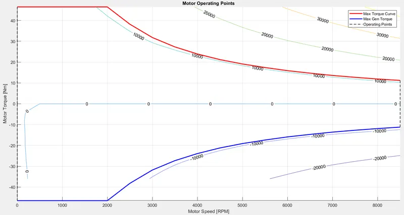
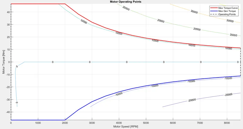
Observation: The motor operating points are within the max torque and regen torque.
Conclusion:
A forward energy-based fuel consumption model of a P1 hybrid vehicle is modeled and successfully simulated in MatLab and Simulink. The fuel economy numbers for both cycles were compared with the conventional vehicle model. The required plots were generated and compared for both cycles. The functionality of the P1 hybrid architecture was learned and understood.