Project 2
AIM: Development of a forward energy-based fuel consumption model of a P1 hybrid vehicle.
- Tabulate the fuel economy numbers (kmpl) for UDDS and HWFET cycle. Compare these numbers with the baseline numbers for conventional vehicle model from Project 1.
Plot the time trace for engine, transmission input, transmission output and wheel speed on one plot.
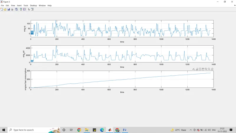
c. Plot engine torque, engine power, fuel rate and fuel consumption using subplots.
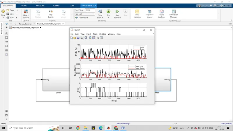
d. Plot accelerator and brake pedal, gear command, vehicle desired and actual speed, vehicle distance using subplots.
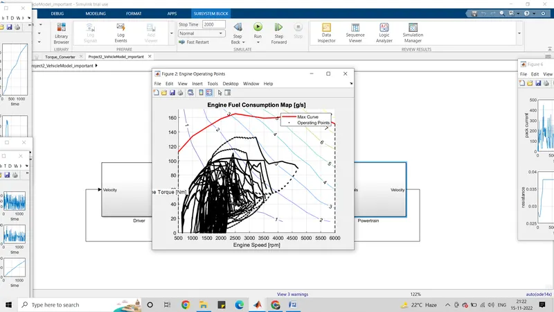
e. Plot the engine operating points on the engine fuel map.
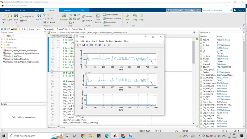
f. Plot motor speed, torque, motor input power using subplots.
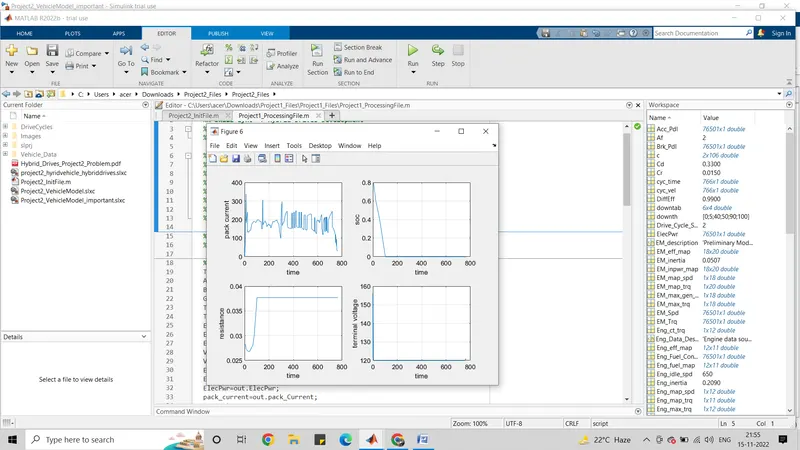
g. Plot pack voltage, current and SoC using subplots.
h. Plot the motor operating points on the motor input power map, with the motor max motoring and generating torque curves.
i. Write down appropriate brief comments on each of these plots, describing the vehicle behavior throughout the drive cycle.
j. Generate the plots for both drive cycles
The hybrid electric vehicle (HEV) P1 reference application represents a full HEV model with an internal combustion engine, transmission, battery, motor, and associated powertrain control algorithms.
the HEV P1 reference application is configured with:
- Lithium-ion battery pack
- Mapped electric motor
- Mapped spark-ignition (SI) engine
This diagram shows the powertrain configuration.
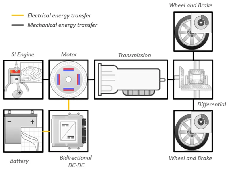
The P1 architecture, with the electric machine connected directly to the crankshaft, is the solution adopted by Honda on their first generation Integrated Motor Assist (IMA) technology. The electric motor functions as a generator, during vehicle deceleration, as an engine starter, and as a motor (to assist the engine) during vehicle accelerations.
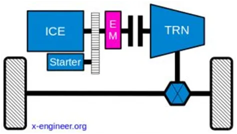
One of the biggest advantage of this solution is that the electric motor can provide higher torque than the BiSG, since there is no belt limitation (due to slip). However, since there is no speed / torque ratio between the electric machine and crankshaft, the torque requirements on the electric motor can be quite demanding.
Two examples of P1 MHEV architectures are:
- Honda Insight Hybrid 2009 (with Integrated Motor Assist technology)
- Mercedes Benz S400 Bluehybrid 2010
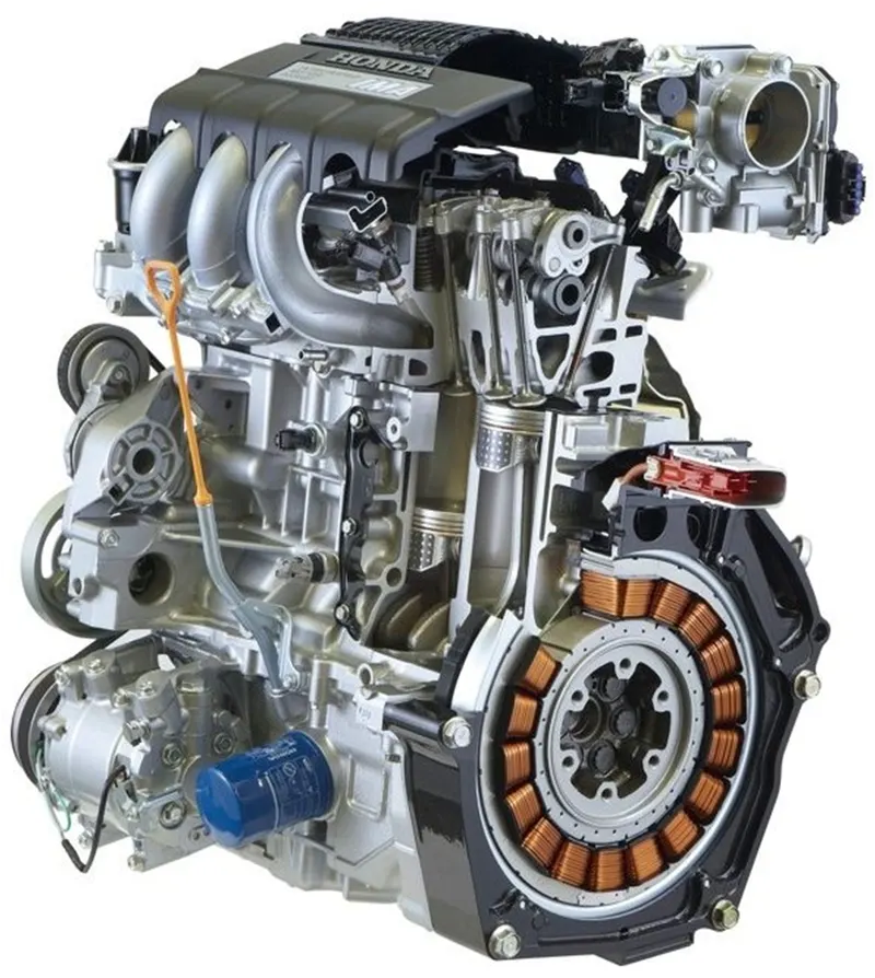
The main characteristics of the crankshaft-mounted electric machine for mild hybrid Honda Insight 2009 are summarized in the table below.
|
Electric machine performance |
Maximum torque (at crankshaft): up to 34 Nm |
|
Hybrid modes (functions) |
Idle Stop & Start |
|
Advantages |
Higher efficiency |
|
Disadvantages |
Output torque limited by the size of the electric machine |
|
Overall characteristics |
Torque Boosting Capability: High (if electric machine is capable) |
The primary advantage of a P1 mild hybrid architecture, compared with P0, is the removal of the belt drive. This means that the efficiency increases a bit (no more belt losses) and the electric machine torque can be higher in terms of amplitude and response (no more belt slip).
The functions (modes) performed by this mild hybrid topology are similar with those of a BiSG (P0), but, overall, P1 configurations have two big disadvantages: higher cost and higher impact on the the existing vehicle architecture. Therefore, vehicle manufacturers and system suppliers are not investing in the further development of crankshaft-mounted integrated starter generator solution for MHEV applications.
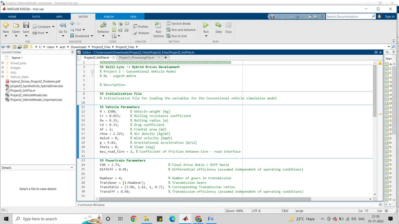
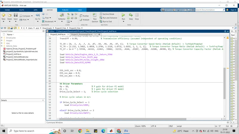
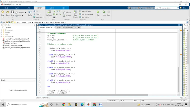
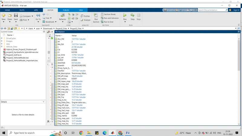
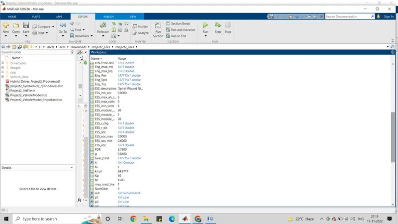
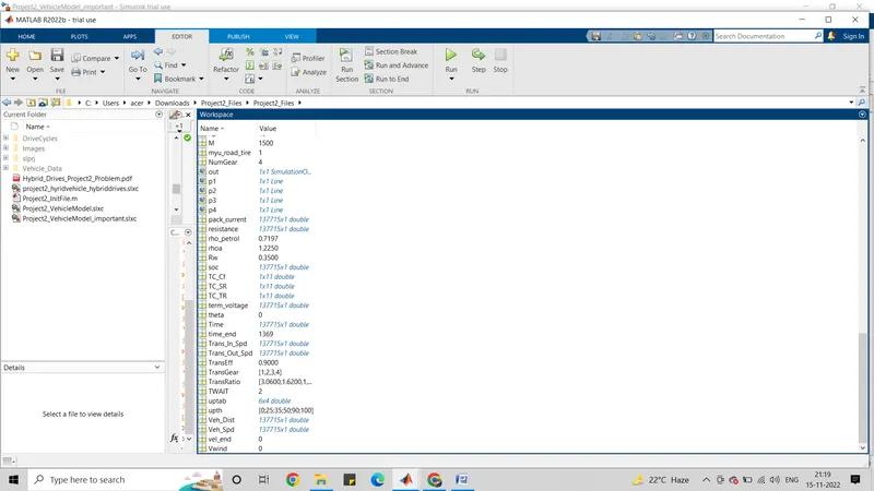
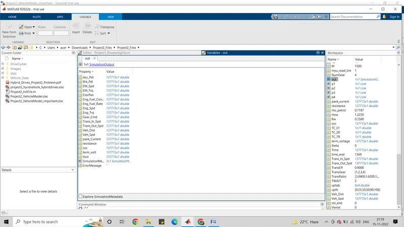
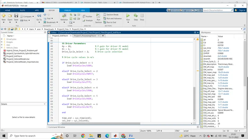
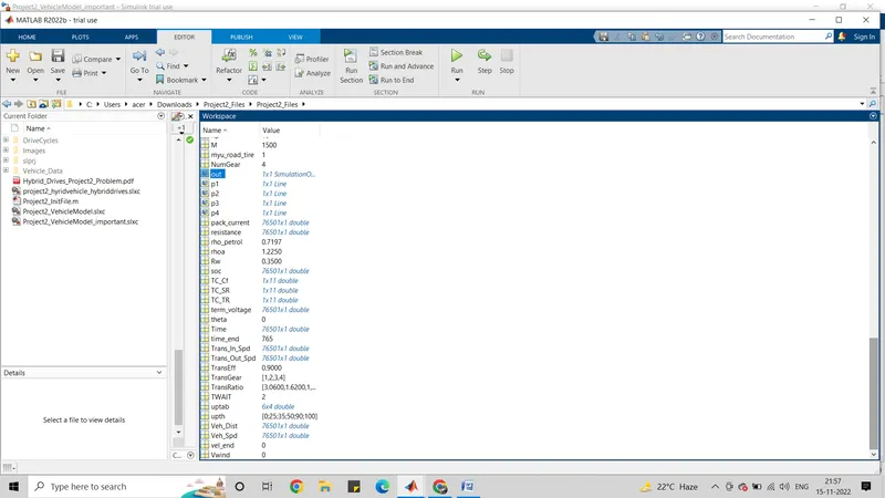
Project2_InitFile.m” is a Matlab script used to load all the variables required for running the Simulink model and for post-processing. The drive cycle selection is also done here. Before running the Simulink vehicle model, run this initialization script.
This is for the UDDS cycle.
simulink model:
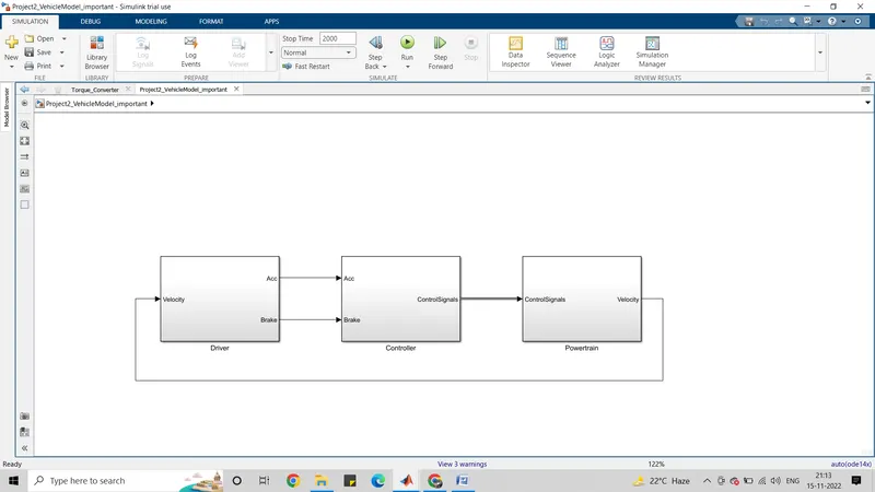
the required drive cycle is fed as input to the driver block and it generates the vehicle acceleration and braking percentage requirements whereby simulating a driver input such that the vehicle is following the required drive cycle.
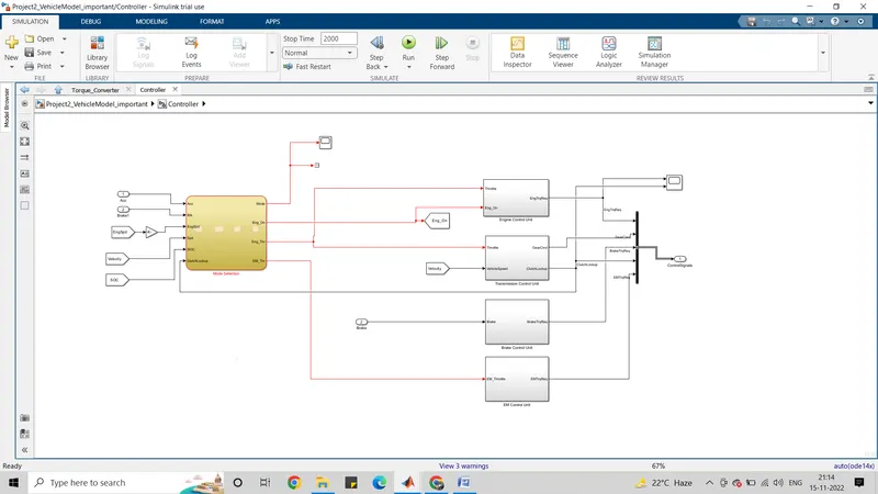
This acceleration and brake percentage requirements is fed onto the controller block which then generated the control signals to meet the driver requirements. The generated control signals are then passed onto the Power train via a bus.
The power train block takes the control signals as input, segregates them and passes them to the appropriate power train components so that the vehicle meets the demands of the driver.
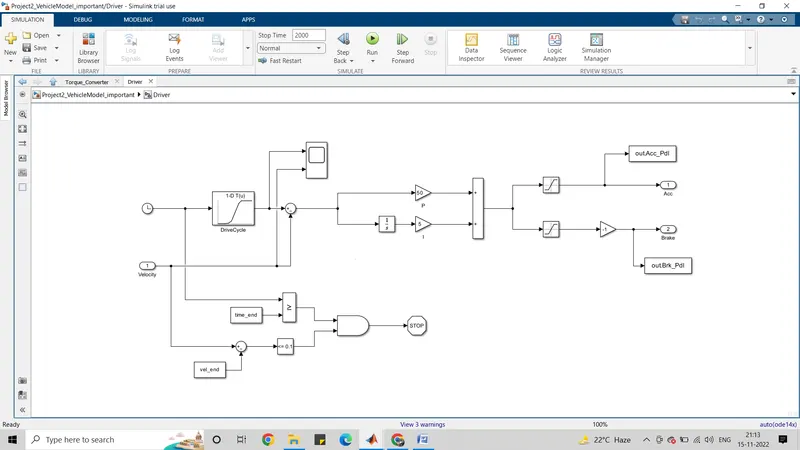
The driver block is essentially a PI controller. It first checks the actual generated velocity from the vehicle with the velocity from the drive cycle with the help of a lookup table. The difference is then passed onto a PI controller which has a gain and integrator block and gives the change in a percentage. This output value from the PI controller can be either positive or negative depending on the current velocity of the vehicle. This value is then saturated to get the required acceleration and braking needs so that the vehicle meets the demands of the driver or in effect the drive cycle. This negative signal for the brake pedal is multiplied by -1 to make it a positive value.
The driver block is also designed to stop the simulation if the simulation meets the end time of the drive cycle and if the velocity of the vehicle is the end velocity of the drive cycle which would basically mean we reached the end of the drive cycle.
Working of state flow:
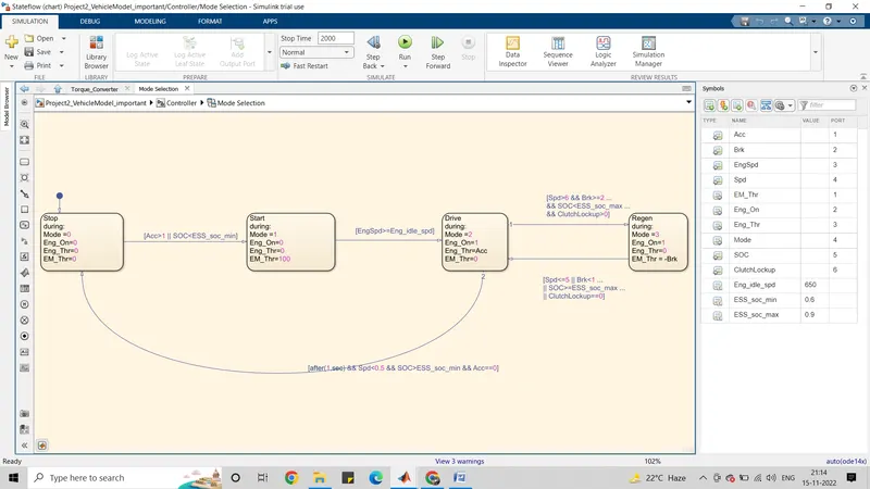
The state flow block takes in various inputs such as engine speed, acceleration and braking requirement, state of charge etc and uses them to determine the mode the vehicle is presently in. The Simulink model includes 4 modes for the vehicle which are described below
Mode 0: Stop
Mode 0 basically simulates the vehicle in the stop condition. Here the engine will be shut off, engine and motor throttle requirement is zero. It is basically used when the vehicle is at a stop signal or stopped for a brief period of time.
Mode 1: Start
Mode 1 is used to signal that the vehicle is needed to be started and moved. As a result, the Electric Motor is turned on and it will be used to start the internal combustion engine for motion. Here since the engine is still in off condition, the engine throttle is zero however motor throttle will be at a hundred percent.
Mode 2: Drive
In this mode, the engine is turned on and the vehicle starts moving. Since the engine is up and running the electric motor is turned off. The acceleration requirements for the vehicle will be solely provided by the engine.
Mode 3: Regenerative braking mode
This mode is used when the vehicle speed and braking requirements are above a certain threshold provided the current SOC is less than the maximum SOC the battery can handle.
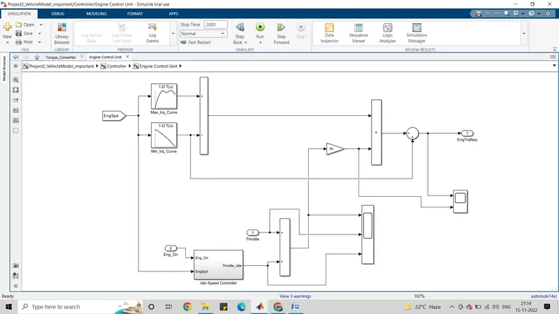
On the basis of the current model, the signals such as whether the engine is on or off, engine throttle and electric motor throttle signals are given to the appropriate control units to convert them into their torque requests to be sent to the power train.
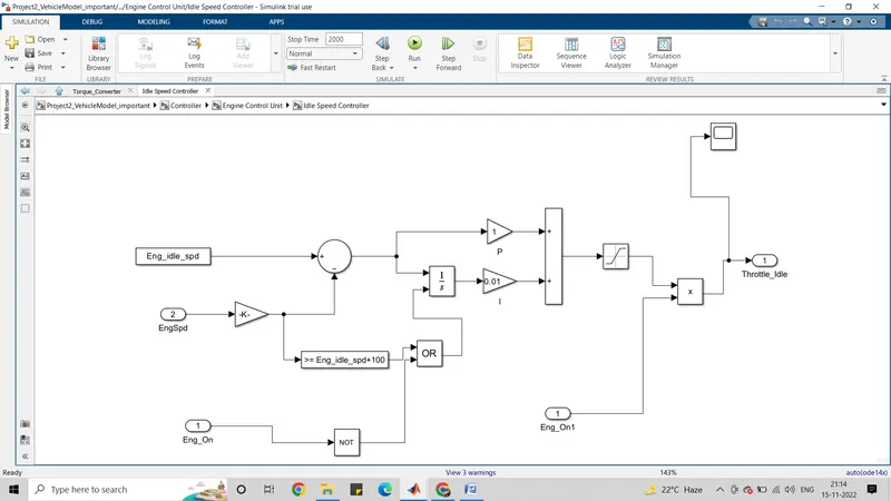
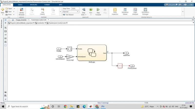
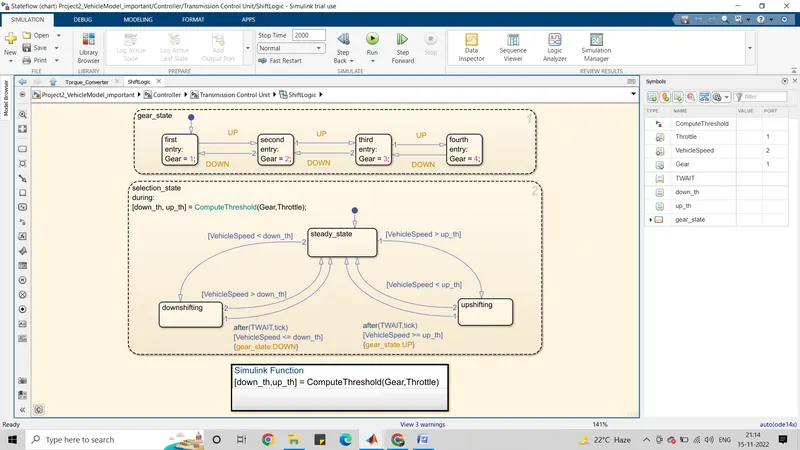
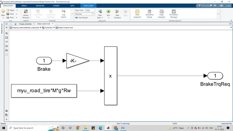
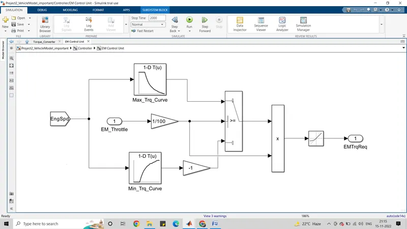
EM control unit: First, it is checked whether the EM throttle is positive or negative. Positive values mean torque is requested from the motor and takes values from the Max torque curve with the help of a 1D look-up table else if the torque is negative, it means torque is being generated by the motor and takes values from the Max generated torque look-up table. This is made possible with the help of a switch block. A negative gain of -1 is given to the generated torque value so that the throttle request remains negative since both EM_throttle and Max generated torque values will be negative.
A rate limiter is also used to control the rate at which the EM torque request increases or decreases because sudden changes in torque values are not desirable.
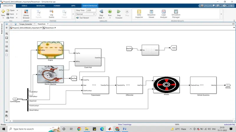
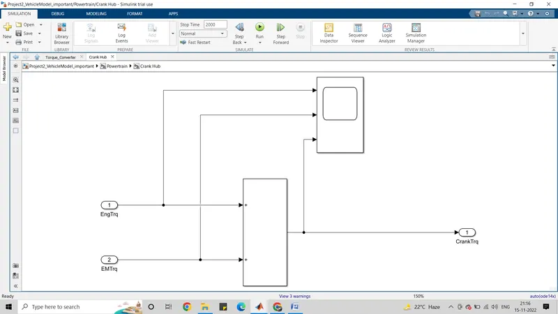
The powertrain block consists of the following subsystems: Engine, Electric mahicne, Crankhub, Energy Storage System, Transmission, Differential, Wheels and Vehicle Dynamics. The signals from the Controller block are extracted using the bus selector, which consists of the signal for Engine torque requirement, Gear command, Brake Torque Requirement, Electric Motor Torque Requirement and Clutch Lockup.
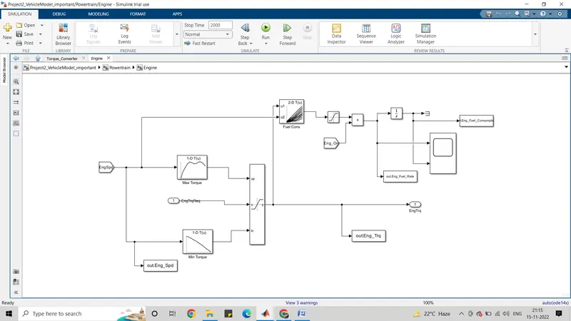
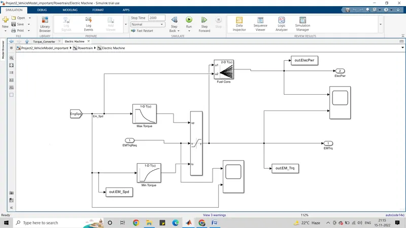
The Electric machine sub-block works almost in the same way as that of the engine block. The E Motor torque request from the control signal is used as input and passed through a dynamic saturation block which takes the upper and lower limits from 1 D lookup tables and gives the required Electric Motor torque as output. These limits are computed with the help of 1-D look-up tables which take engine speed or E-Motor speed (here both are the same as in this P-1 architecture, the e motor is directly coupled to the engine without a clutch in between) as inputs. E Motor speed and E Motor generated torque is passed to a 2-D lookup table which gives the produced (in case of motoring) or generated (in case of regenerative braking) electric power. The required parameters are transferred to the workspace using To Workspace blocks.
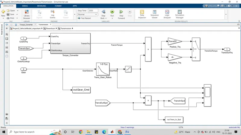
The transmission block takes Crank Torque, Clutch Lockup and Gear Command as input and computes transmission input torque with the help of a torque converter block. This Input transmission torque is then passed onto a gear system which uses the gear ratio to calculate the transmission output torque and transmission input speed. The gear ratio is selected with the help of a 1-D lookup table. The switch is used in order to consider the efficiency of the transmission.
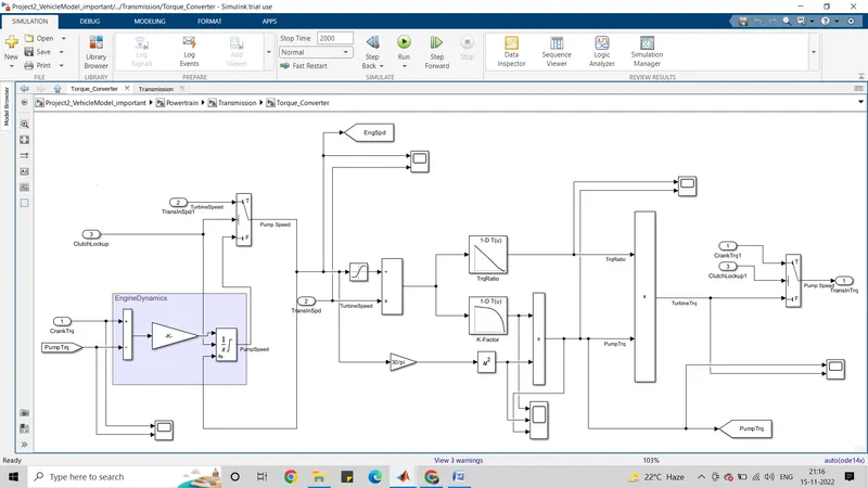
A torque converter is used because when the vehicle is stopped the engine speed can not go below a particular value as that will result in engine stalling. So the engine must keep spinning at minimum idle speed. In addition, when torque is to be transmitted from the crank hub to the transmission unit, it needs to be smooth otherwise a lot of vibrations will be produced. A torque converter also provides torque multiplication at low speeds. The fluid in the torque converter ensures a smooth transfer of torque from the engine to the transmission unit. The torque converter takes in crank torque, clutch lockup signal and transmission input speed as inputs.
First, the pump torque is subtracted from crank hub torque as that is the load on the engine. The subsequent value is then divided by the sum of the engine and electric motor inertia to get the acceleration. This value is then integrated to get the pump speed. A switch is used to determine whether the pump speed is the aforementioned calculated value or the turbine speed (in case of clutch lockup is 1).
The turbine speed is divided by the pump speed to get the speed ratio which is passed as input to 1-D lookup tables to get the corresponding torque ratio and capacity factor.
The capacity factor is used for finding the pump torque from the pump speed using the equation,
C factor = pump torque/pump speed
C factor=pump torque in Nmpump speed in rpm2C factor=pump torque in Nmpump speed in rpm2
This pump torque is used to find the turbine torque using the torque ratio.
A switch is used at the end to ensure that if the clutch lockup signal is 1 then transmission input torque will be the crank hub torque since during clutch lockup crank hub torque will be directly transmitted to the turbine.
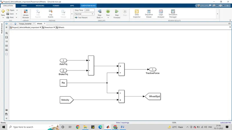
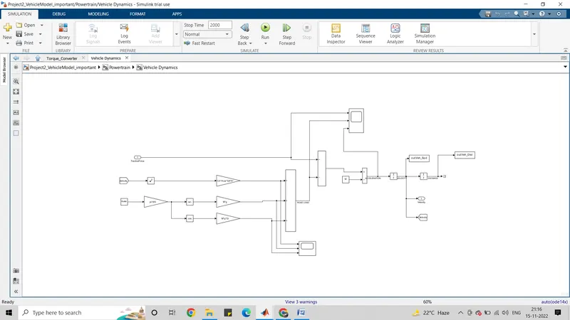
The Vehicle Dynamics block is used to determine the resultant vehicle velocity and the distance travelled. This is done by calculating the resultant force acting on the vehicle by subtracting the road load from the tractive force on the vehicle.
The road load is divided into three components i.e drag force, rolling resistance and gradient resistance.
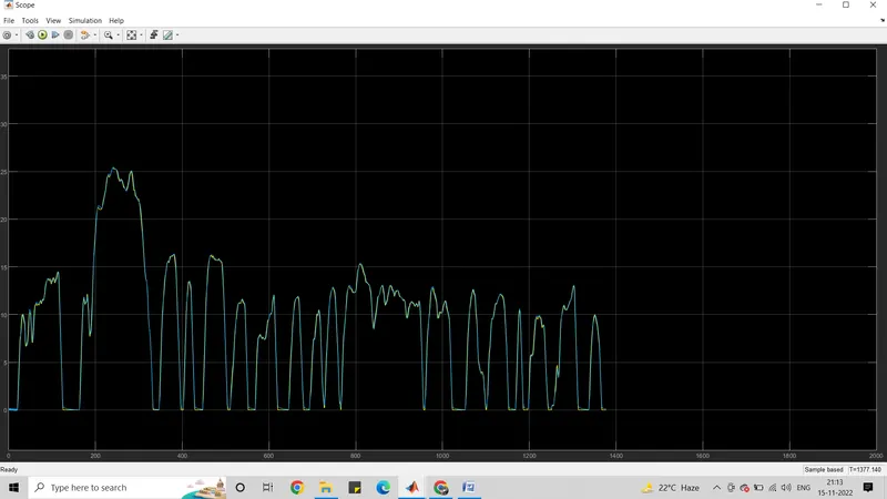
After calculating the resultant force acting on the vehicle, the value is divided by the vehicle mass to get the vehicle acceleration which is then integrated to get the vehicle velocity which upon integration gives the distance travelled by the vehicle. The sample output from the scope for the UDDS drive cycle is shown in Figure 9. The longitudinal dynamics equation which is used for the respective block is, MdVdt=ηtλTmRw−(12ρaAfCd(V±Vw)2+CrMgcosθ+Mgsinθ)MdVdt=ηtλTmRw-(12ρaAfCd(V±Vw)2+CrMgcosθ+Mgsinθ)
where, ρais the air density, Af is the frontal area, Cd is the drag coefficient, VV is the vehicle speed, Vw is the wind speed, Cr is the rolling resistance coefficient, MM is the vehicle mass, gg is the gravity constant, θθ is the road grade, ηt is the transmission efficiency, λλ is the final drive ratio, Tmis the input transmission torque and Rw is the wheel radius.
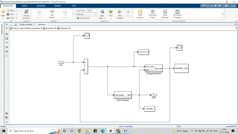
This sub-block takes electrical power generated by the E-motor as input and calculates the state of charge (SOC) of the battery pack. The SOC increases if the E-Motor is generating power and decreases if the E-Motor is producing motoring power.
The electrical power is divided by the terminal voltage to get the pack current which is then used to calculate the SOC. Terminal voltage is calculated by an equivalent circuit model.
SOC estimation: This block takes in pack current as input and calculates the SOC. Pack current is first passed through an integrator block to get the total current passed during the time period in Ampere seconds or Coulombs. A gain block is used to convert this value into Ampere hours. This capacity of charge is then divided by the maximum capacity of the battery to get the fraction of SOC used (positive) or gained (negative). This value is then added to the initial SOC value and saturated between 1 and 0 to get the current SOC value. 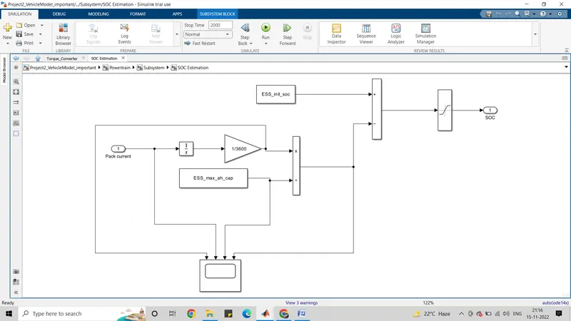
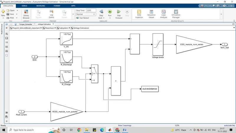
TERMINAL VOLTAGE: This sub-block takes in the pack current and SOC of the battery as input and calculates the Terminal voltage of the battery pack as the output using the equivalent circuit model.
The SOC value is passed through three 1-D lookup tables to calculate the corresponding open circuit voltage and module resistance during charging and discharging. A switching block is used to choose the appropriate module resistance during charging or discharging based on the sign of the module current. I.e if module current is positive. The model will take the discharge resistance value and vice versa. The pack current is divided by the number of modules in parallel to get the current passing through each module. The calculated module resistance is multiplied by the module current and the resultant value is subtracted from the open circuit voltage to get the module terminal voltage as per the following equation.
Vterminal=VOC−IRVterminal=VOC-IR
The calculated terminal voltage of the module is then multiplied by the number of modules in series in the battery pack to get the pack terminal voltage.
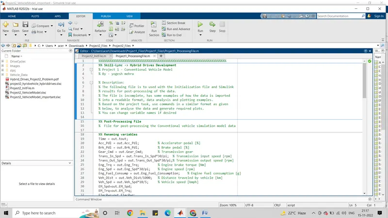
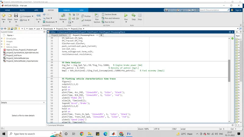
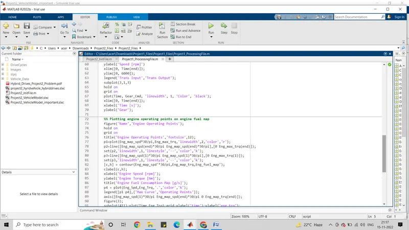
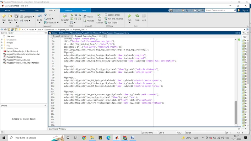
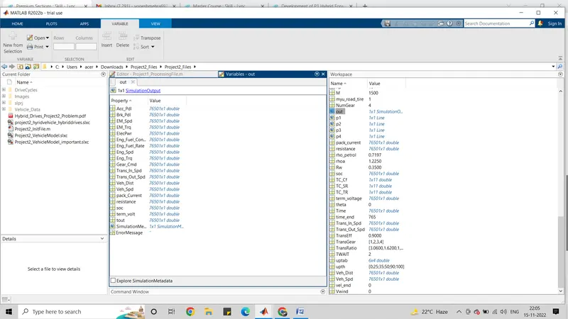
Then we have to run the processing 1 file to plot the figures .
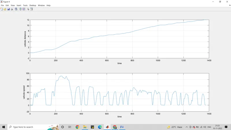
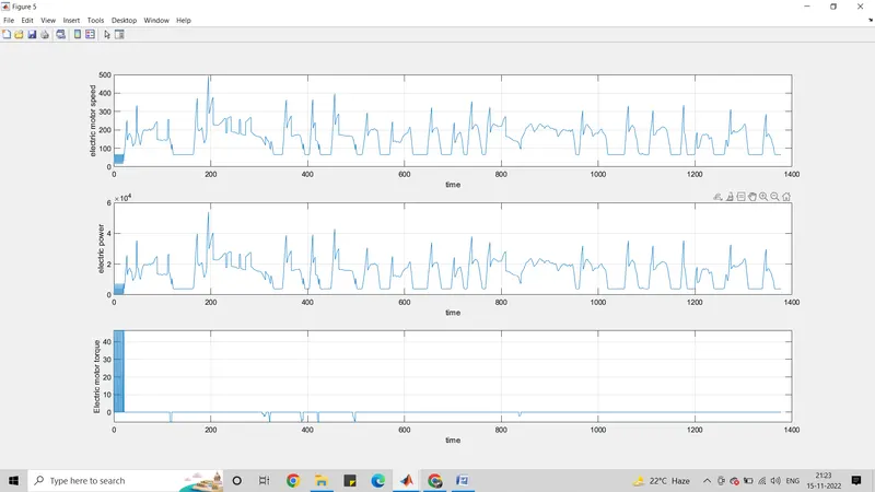
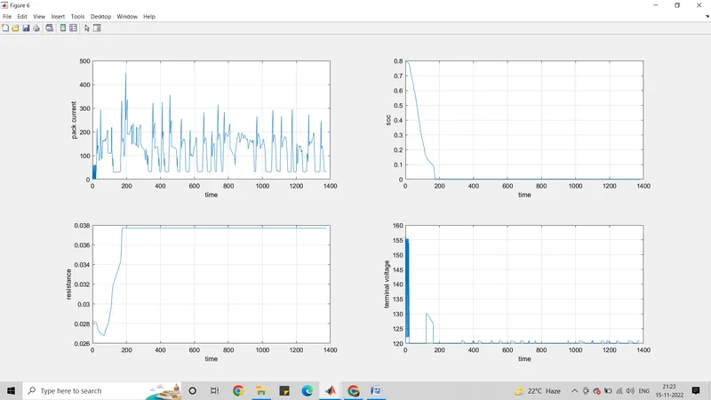
THIS IS FOR HWFET(HIGHWAY CYCLE).
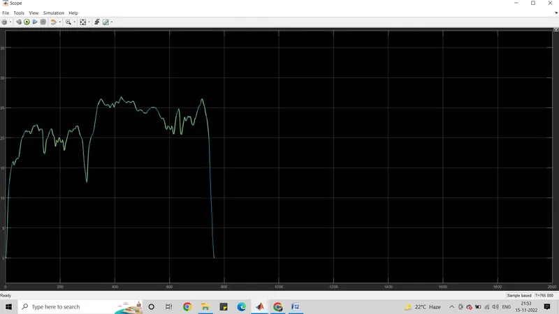
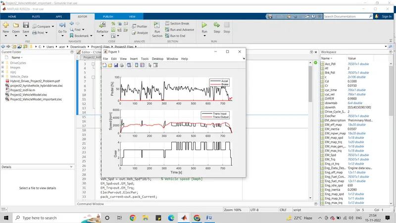
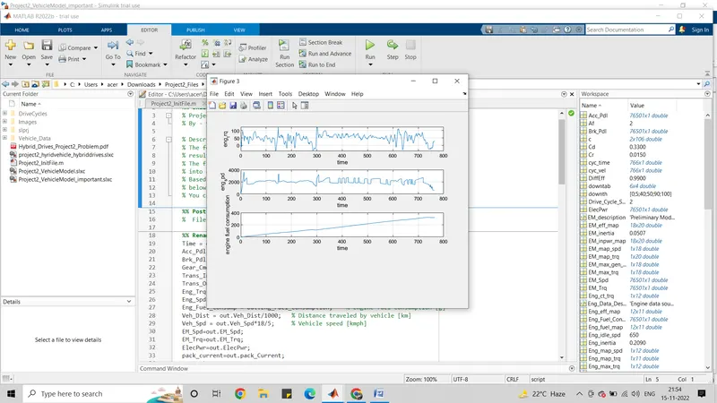
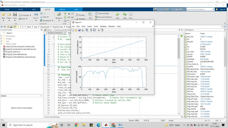
CONCLUSION: The fuel economy seemed to be significantly more for the HWFET drive cycle than the UDDS for the same vehicle characteristics.
The comparative study of UDDS and HWFET for the developed vehicle model is analyzed and it was found that the P1 hybrid architectures have better fuel economy as compared to conventional vehicles.