Project 1
AIM. The task of this project is to compute the fuel economy numbers for the given vehicle (kmpl) on the urban cycle (UDDS) and highway cycle (HWFET). Also, to analyze and understand the vehicle operating
points in terms of engine speed, torque, transmission speeds, pedal positions, gear, distance traveled, etc.
OBJECTIVES: a. Tabulate the fuel economy numbers (kmpl) for UDDS and HWFET cycle. This forms the baseline numbers for comparing with the future hybrid version.
b. Plot the time trace for engine, transmission input, transmission output and wheel speed on one plot.
c. Plot engine torque, engine power, fuel rate and fuel consumption using subplots.
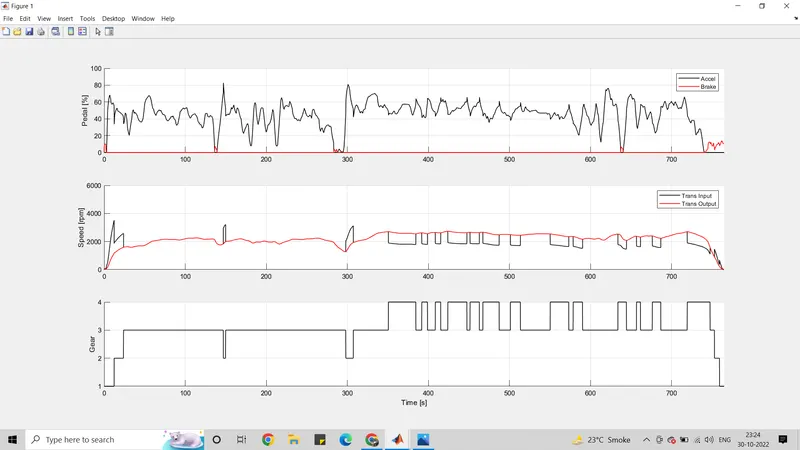
d. Plot accelerator and brake pedal, gear command, vehicle desired and actual speed, vehicle distance using subplots.
e. Plot the engine operating points on the engine fuel map.
f. Write down appropriate brief comments on each of these plots, describing the vehicle behavior throughout the drive cycle.
g. Generate the plots for both drive cycles
THEORICITAL CONCEPTS REGARDING FORWARD ENERGY MODEL OF CONVENTIONAL VEHICLE:
A driver controller is required to control the vehicle to follow a desired speed and set the start of the calculations. The controller is implemented to model the driver that will either push the accelerator or the brake pedal to match the desired speed which enables to study the driver behaviour. The controller is used as part of a feedback loop that will determine the energy required to drive the vehicle.
Vehicle Energy Consumption Estimation Models
- Analytical models:
Analytical models are representative of the Vehicle behaviour and can be developed in MATLAB/Simulink by creating an vehicle model. They are based on fundamental theoretical equations. A model of the vehicle dynamics is built based on vehicle dynamics theory to calculate the power required at the wheels to overcome the resistances forces opposed to the vehicle motion: Aerodynamic Drag, Rolling, Inertia, Gradient and Transmission resistances. The power required derives from the tractive force expressed as the sum of the resistances forces above
- Statistical models:
Statistical models are built based on real world driving data analysis to derive empirical relationships between the different factors affecting Vehicles energy consumption.
- Computational models:
There are mainly two kinds of computational models for energy consumption estimation: Artificial Neural Networks (ANN) based model. Clustering based models
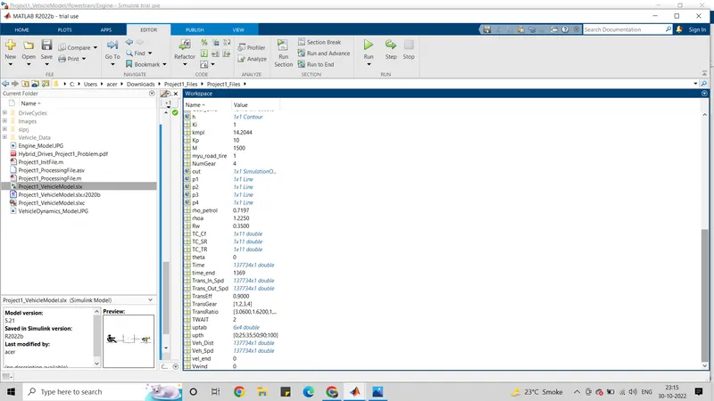
- FOR UDDS: The matlab initilization file and procession file are in screeshot itself. the workspace values are also in screenshot itself.
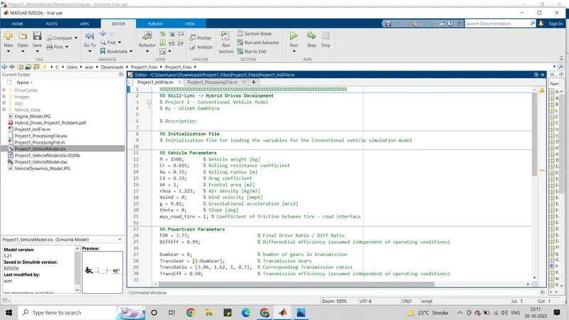
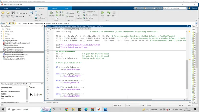
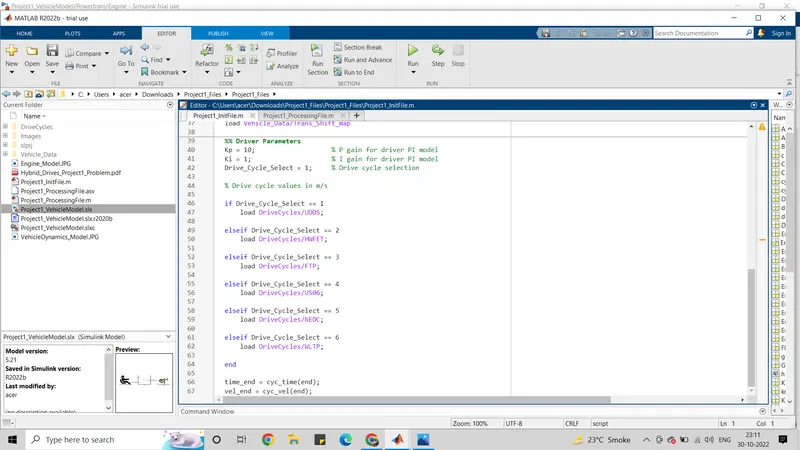
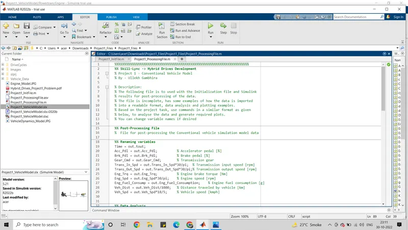
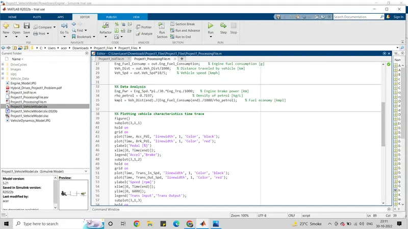
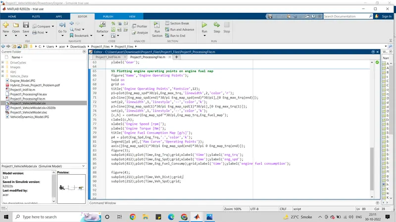
we can change the drive cycle by changing the drive cycle values:
- The Drive Cycle can be selected from this MATLAB Script, By changing the variable Drive_Cycle_Select to,
| 1 | UDDS |
| 2 | HWFET |
| 3 | FTP |
| 4 | US06 |
| 5 | NEDC |
| 6 | WLTP |
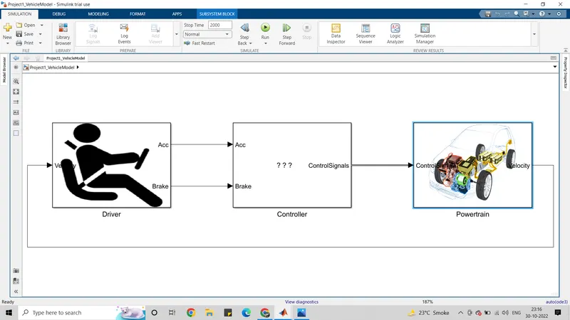
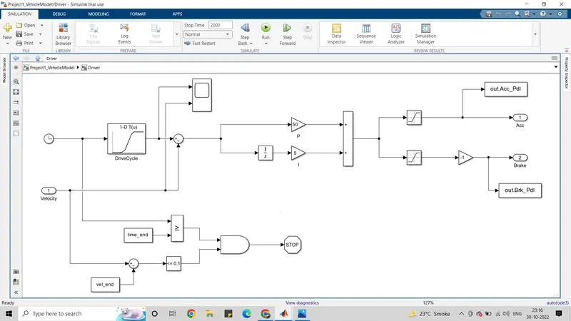
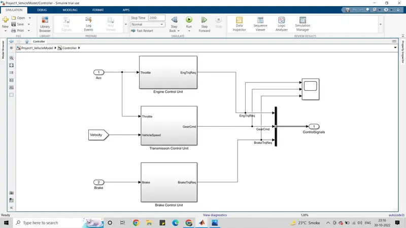
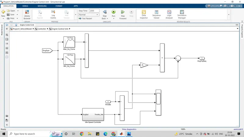
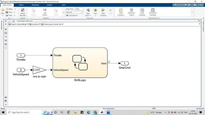
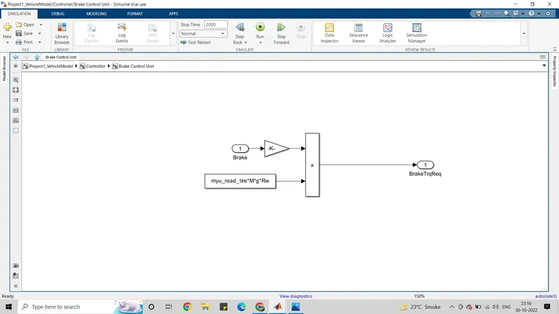
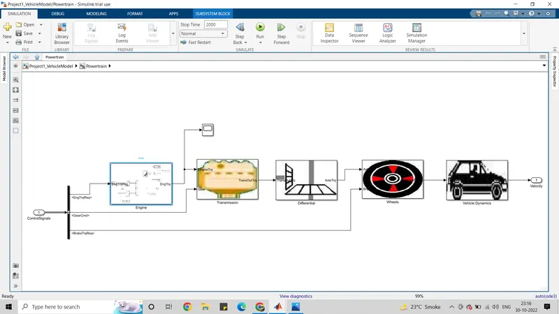
ENGINE MODEL DESCRIPTION:
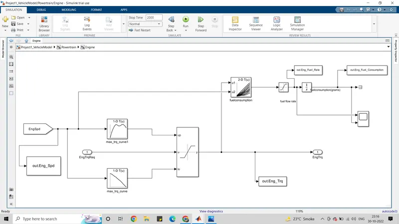
- Based on the Engine speed The required torque from the controller is saturated between Max torque curve and min torque curve and passes the Engine torque to the Transmission block
- The 2D lookup table is used to calculate the fuel flow rate based on engine speed and engine torque. The fuel flow rate is then integrated to find the fuel consumption.
- Estimated fuel flow rate, fuel consumption, engine torque and engine speed are passed to the MATLAB workspace using the to-workspace block.
- Engine fuel flow rate and Fuel consumption are scoped.
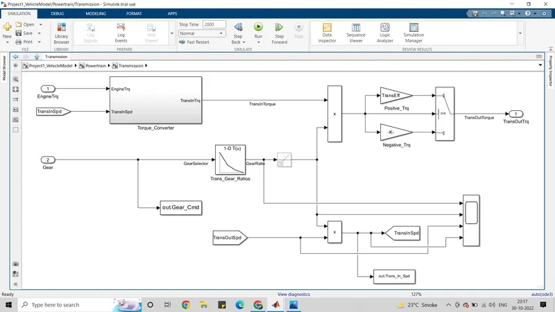
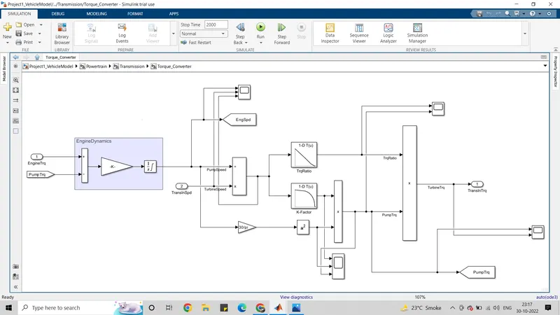
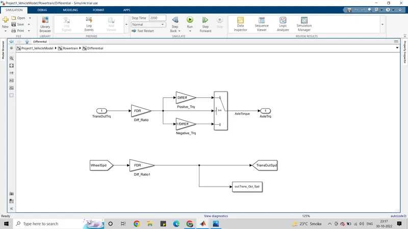
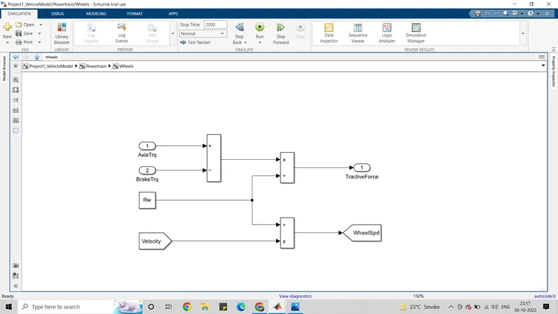
VEHICLE DYNAMICS: In this takes tractive force and road load. It is dictates vehicle speed based on tractive force and road load.
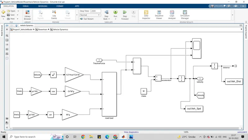
- Tractive Force and Road loads are used to calculate the vehicle velocity,
ηt⋅λt⋅TeRw=MdVvehdt+12ρaAfCd(Vveh+Vwd)2+CrMgcosθ+Mgsinθηt⋅λt⋅TeRw=MdVvehdt+12ρaAfCd(Vveh+Vwd)2+CrMgcosθ+Mgsinθ
ηt⋅λt⋅TeRwηt⋅λt⋅TeRw = Tractive force
12ρaAfCd(Vveh+Vwd)2+CrMgcosθ+Mgsinθ12ρaAfCd(Vveh+Vwd)2+CrMgcosθ+Mgsinθ = Road Load
Where,
ρ a - Air Density
A f - Frontal Ares
C d - Drag Coefficient
C r - Rolling Coefficient
M - Mass of Vehicle
g - Acceleration due to gravity
θ - Slope
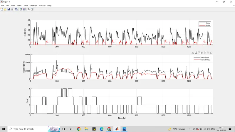
SIMULATION RESULT OF UDDS CYCLE:
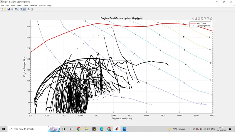
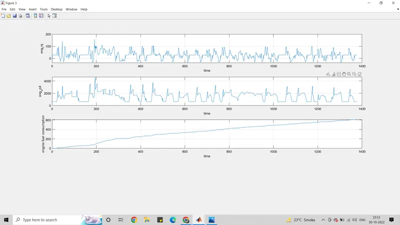
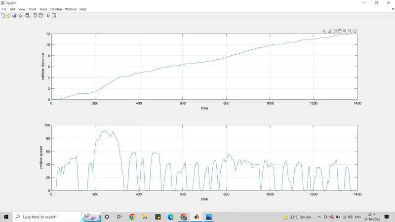
SIMULATION FOR HWFET CYCLE:
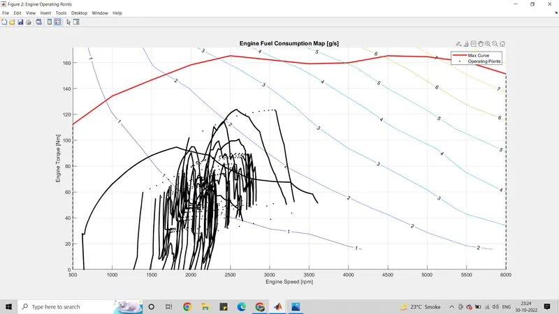
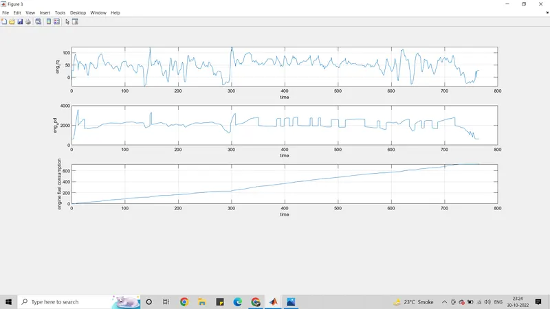
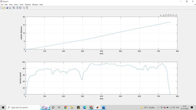
WORKSPACE FOR UDDS CYCLE: By which we can compare kmpl values
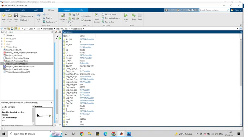
WORKSPACE FOR HWFET CYCLE:
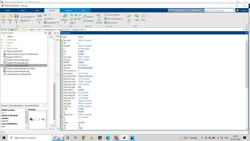
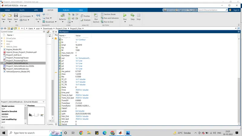
IF WE COMPARE THE KMPL VALUES FOR UDDS AND HWFET CYCLE WE CAN SEE THAT KMPL IS MORE FOR HWFET BECAUSE IT HAVE MINIMUM IDLE LOSSES AND BREAKING IS NOT FREQUENT IN HIGHWAY CYCLE SO IT ULTIMATELY COMES UNDER MORE FUEL CONSUMPTION.
THE DESCRIPTION OF OTHER SUBSYSTEM ARE NOT NEEDED RIGHT IN OUR CASE .
CONCLUSION
- Hence, the forward energy-based fuel consumption model of a conventional vehicle has been successfully Simulated using MATLAB and Simulink.
- Analyses and understands vehicle operating points based on engine speed, torque, transmission speed, pedal positions, gear, and distance travelled.
- Post process calculations were performed and the required graphs were successfully plotted.
- Successfully calculated vehicle fuel efficiency numbers (kmpl) for the given city cycle (UDDS) and highway cycle (HWFET)