Challenge

Project 2

SSubhadeep Kundu4 Nov 2022

P1 Hybrid Architecture

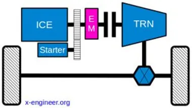
Positioned between the engine and transmission, the P1 hybrid architecture and High Voltage Integrated Starter Generators (HV ISG) enable high-efficiency power generation while featuring regenerative braking and acceleration assist.

One of the biggest advantages of this solution is that the electric motor can provide higher torque than the BiSG, since there is no belt limitation (due to slip). However, since there is no speed / torque ratio between the electric machine and crankshaft, the torque requirements on the electric motor can be quite demanding.

FEATURES AND BENEFITS

Permanent magnet rotor
BorgWarner S-wind stator technology
Air/oil/WEG cooling options available
Highly adaptable to different voltage, torque and power requirements

Two examples of P1 MHEV architectures are:

Honda Insight Hybrid 2009 (with Integrated Motor Assist technology)
Mercedes Benz S400 Bluehybrid 2010

Simulink Model:

Vehicle Model:

Driver Model:

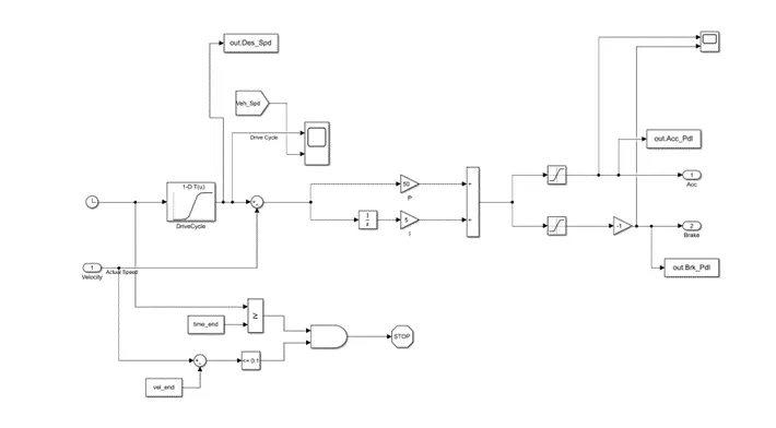
A driver model is a mathematical model which replicates the functionality of a driver

(controlling , monitoring and stabilizing a vehicle) during various manoeuvres . In this case, it a PI controller is a basic PI controller that generates accelerator and brake pedal outputs to match the desired and actual vehicle speeds.

Controller Model:

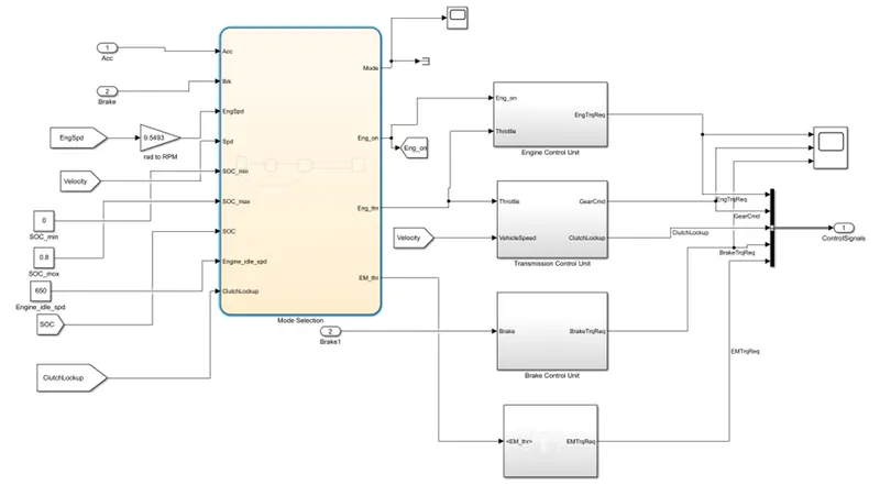
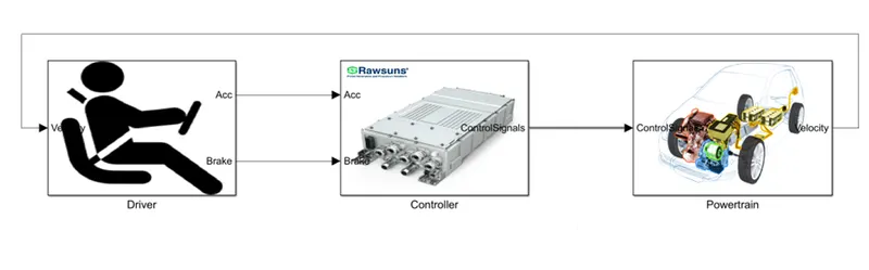
The Controller block represents the electronic controls units. It is based on the driver inputs, it generates desired engine torque, desired transmission gear and desired brake torque. These inputs are fed to the ‘Powertrain’ block which represents the drivetrain of the vehicle.

Mode Selection:

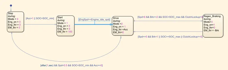
The state flow model is used to represent the supervisory control unit, which decides the operation mode while it is in start, stop mode, cruising mode or regen braking mode.

The inputs are acceleration, Brake, Engine Speed in RPM, Velocity, SOC_min, SOC, SOC_max, Engine idle speed and Clutch Lockup.

The 1^st, 2^nd, 3^rd and 4^th blocks represent Stop, Start, Drive and Regen Braking respectively.

The outputs are operation mode, engine on/off, engine throttle, motor throttle.

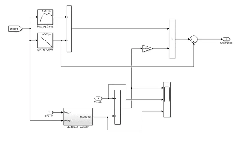
Engine Control Unit:

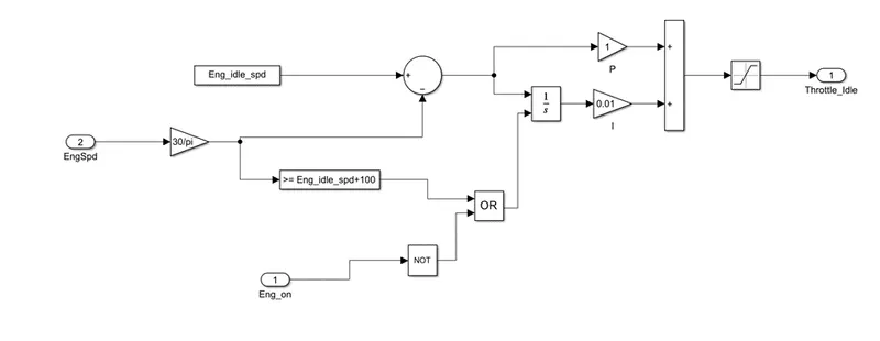
Idle Speed Controller:

Transmission Control Unit:

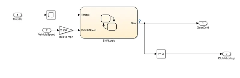
The transmission control block controls the gear shifting by using the study ShiftLogic chart.

Brake Control Unit:

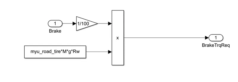
Brake Control unit gives the required brake torque according to the brake pedal input.

Motor Control Unit:

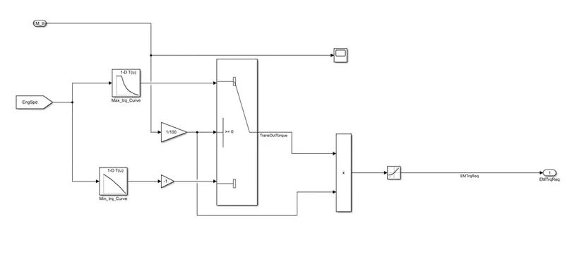
Motor Control Unit estimates the Motor Torque required by comparing the EM_throttle with the lookup tables.

Power Train:

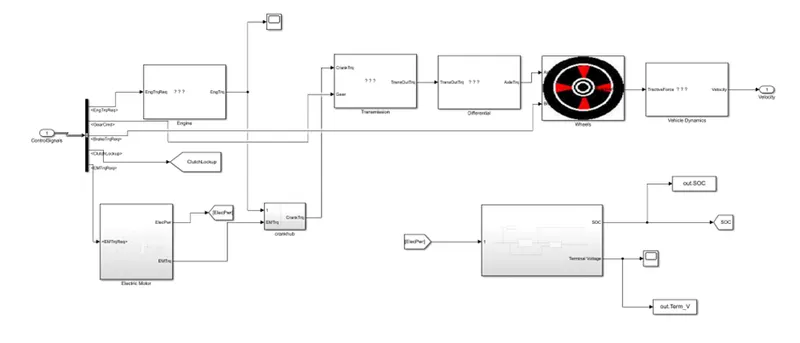
The control signals from the control model are transmitted via a bus to the corresponding blocks in the powertrain model. The powertrain model includes all the components that convert the power of the engine into vehicle motion.

The components are: Engine, Battery Pack, Electric Motor, Crank Hub, Transmission, Differential, Wheels and the vehicle body dynamics subsystems.

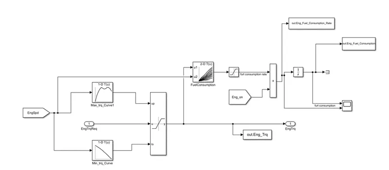
Engine:

Electric Motor:

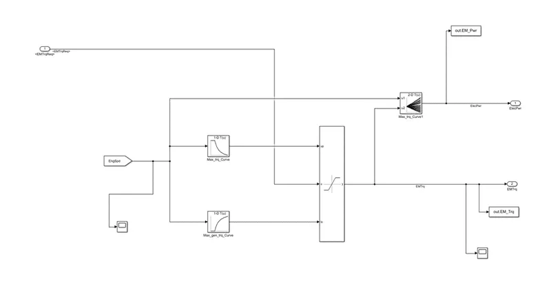
Crank hub:

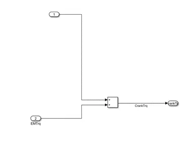
Crank Hub adds up the EM torque and the Engine torque and gives output to the transmission block as the crank torque.

Transmission:

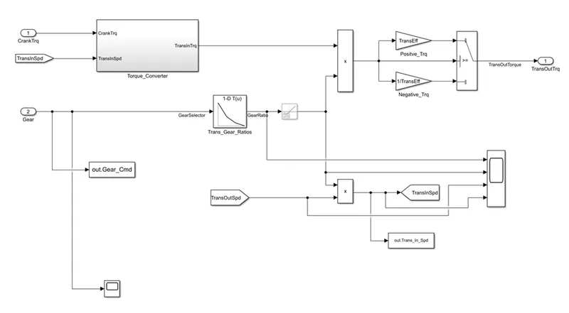
Torque Converter:

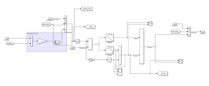
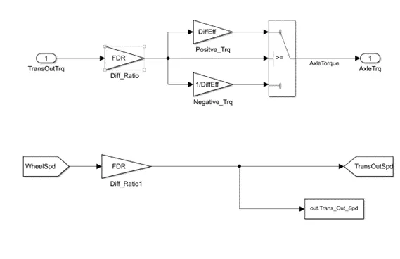
Differential:

Wheels:

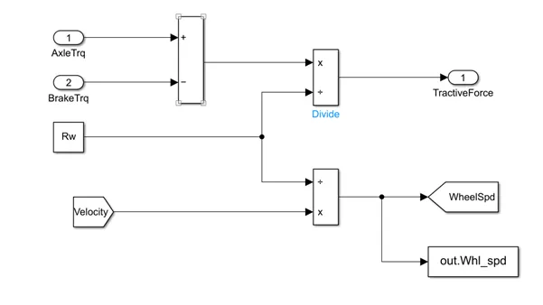
Vehicle Dynamics:

Equations for aerodynamic drag, rolling resistance, and gradient are implemented and added using simulink blocks to get road load.

Road load is subtracted from the tractive force to get the inertia force. Inertia force is then divided by the mass to get the acceleration.

Acceleration is integrated to get speed which is again integrated to get distance travelled.

Speed is used in the closed loop operation.

'To workspace' blacks are implemented in the models for further calculations and plotting.

Pre processing:

MATLAB code:

%% Initialization File

% Initialization file for loading the variables for the Conventional vehicle simulation model

%% Vehicle Parameters

M = 1500; % Vehicle weight [kg]

Cr = 0.015; % Rolling resistance coefficient

Rw = 0.35; % Rolling radius [m]

Cd = 0.33; % Drag coefficient

Af = 2; % Frontal area [m2]

rhoa = 1.225; % Air density [kg/m3]

Vwind = 0; % Wind velocity [kmph]

g = 9.81; % Gravitational acceleration [m/s2]

theta = 0; % Slope [deg]

myu_road_tire = 1; % Coefficient of friction between tire - road interface

%% Powertrain Parameters

FDR = 3.73; % Final Drive Ratio / Diff Ratio

DiffEff = 0.99; % Differential efficiency (assumed independent of operating conditions)

NumGear = 4; % Number of gears in transmission

TransGear = [1:NumGear]; % Transmission Gears

TransRatio = [3.06, 1.62, 1, 0.7]; % Corresponding Transmission ratios

TransEff = 0.90; % Transmission efficiency (assumed independent of operating conditions)

TC_SR = [0, .5, .6, .7, .8, .87, .92, .94, .96, .97, 1]; % Torque Converter Speed Ratio (Matlab default) -> TurbSpd/PumpSpd

TC_TR = [2.232, 1.5462, 1.4058, 1.2746, 1.1528, 1.0732, 1.0192, 1, 1, 1, 1]; % Torque Converter Torque Ratio (Matlab default) -> TurbTrq/PumpTrq

TC_Cf = 1e-4 * [.72558, .66322, .63463, .59042, .51331, .4144, .29287, .22444, .12186, .04386, 0]; % Torque Converter Capacity Factor (Matlab default) -> PumpTrq/PumpSpd^2 [Nm/rpm^2]

load Vehicle_Data/Engine_data_1_9L_Saturn_95kW

load Vehicle_Data/Trans_Shift_map

load Vehicle_Data/EM_Honda_Insight_10kW

load Vehicle_Data/ESS_NiMH6

ESS_init_soc = 0.8;

ESS_soc_max = 0.9;

ESS_soc_min = 0.6;

%% Driver Parameters

Kp = 10; % P gain for driver PI model

Ki = 1; % I gain for driver PI model

Drive_Cycle_Select = 1; % Drive cycle selection

% Drive cycle values in m/s

if Drive_Cycle_Select == 1

load DriveCycles/UDDS;

elseif Drive_Cycle_Select == 2

load DriveCycles/HWFET;

elseif Drive_Cycle_Select == 3

load DriveCycles/FTP;

elseif Drive_Cycle_Select == 4

load DriveCycles/US06;

elseif Drive_Cycle_Select == 5

load DriveCycles/NEDC;

elseif Drive_Cycle_Select == 6

load DriveCycles/WLTP;

end

time_end = cyc_time(end);

vel_end = cyc_vel(end);

Initializing Battery:

load Pack_Current_test.mat;

load ESS_NiMH6.mat;

ipack_simulink = [t I_pack];

Post Processing:

% Variables

Time = out.tout;

Acc_Pdl = out.Acc_Pdl; % Accelerator pedal [%]

Brk_Pdl = out.Brk_Pdl; % Brake pedal [%]

Gear_Cmd = out.Gear_Cmd; % Transmission gear

Trans_In_Spd = out.Trans_In_Spd*30/pi; % Transmission input speed [rpm]

Trans_Out_Spd = out.Trans_Out_Spd*30/pi;% Transmission output speed [rpm]

Eng_Trq = out.Eng_Trq; % Engine brake torque [Nm]

Eng_Spd = out.Eng_Spd*30/pi; % Engine speed [rpm]

Eng_Fuel_Consump = out.Eng_Fuel_Consumption; % Engine fuel consumption [g]

Desired_Spd = out.Des_Spd;

Veh_Dist = out.Veh_Dist/1000; % Distance traveled by vehicle [km]

Veh_Spd = out.Veh_Spd*18/5; % Vehicle speed [kmph]

Wheel_Speed = out.Whl_spd*18/5; % Wheel speed [kmph]

Eng_Fuel_Rate = out.Eng_Fuel_Consumption_Rate;% Engine fuel rate [%]

Eng_Fuel_Consumption = out.Eng_Fuel_Consumption;

EM_Power = out.EM_Pwr; % Electric Motor Power

EM_Torque = out.EM_Trq; % Electric Motor Torque

EM_Speed = out.EM_Spd*30/pi; % Electric Motor Speed [rpm];

Term_Volt = out.Term_V; % Terminal Voltage of battery

Soc = out.SOC; % State Of Charge

Pack_Current = out.I; % Battery pack current

% Data Analysis

Eng_Pwr = Eng_Spd.*Eng_Trq/1000; % Engine brake power [kW]

% Plotting the time trace for engine, transmission input, transmission output and wheel speed

figure(1)

hold on

grid on

plot(Time, Trans_In_Spd, 'linewidth', 1, 'Color', 'red');

plot(Time, Trans_Out_Spd, 'linewidth', 1, 'Color', 'blue');

plot(Time, Wheel_Speed, 'linewidth',1, 'color', 'black')

ylabel('Speed [rpm]')

xlabel('Time [s]')

legend('Trans Input','Trans Output','Wheel Speed');

% Plotting engine torque, engine power, fuel rate and fuel consumption

figure(2)

subplot(4,1,1)

plot(Time,Eng_Trq,'linewidth',1,'color','black')

xlim([0, Time(end)]);

xlabel('Time [s]')

ylabel('Torque [Nm]')

legend('Engine Torque')

grid on

subplot(4,1,2)

plot(Time,Eng_Pwr,'linewidth',1,'color','blue')

xlim([0, Time(end)]);

xlabel('Time [s]')

ylabel('Power [KW]')

legend('Engine Power')

grid on

subplot(4,1,3)

plot(Time,Eng_Fuel_Rate,'linewidth',1,'color','red')

xlim([0, Time(end)]);

xlabel('Time [s]')

ylabel('Fuel Rate [%]')

legend('Engine Fuel Rate')

grid on

subplot(4,1,4)

plot(Time,Eng_Fuel_Consumption,'linewidth',1,'color','green')

xlim([0, Time(end)]);

xlabel('Time [s]')

ylabel('Fuel Consumption')

legend('Engine Fuel Consumption')

grid on

% Potting Accelerator pedal, Brake pedal and gear command with respect to time

figure(3)

subplot(4,1,1)

hold on

plot(Time, Acc_Pdl, 'linewidth', 1, 'Color', 'blue');

plot(Time, Brk_Pdl, 'linewidth', 1, 'Color', 'red');

ylabel('Pedal [%]')

xlabel('Time [s]');

xlim([0, Time(end)]);

grid on

legend('Accel','Brake');

title('Acceleration & Brake Pedal wrt Time')

subplot(4,1,2)

plot(Time(1:19126), Gear_Cmd, 'linewidth', 1, 'Color', 'black');

xlabel('Time [s]');

ylabel('Gear');

grid on

title('Gear command wrt Time')

subplot(4,1,3)

plot(Time,Desired_Spd*18/5, 'linewidth', 1, 'Color', 'green');

xlabel('Time');

ylabel('Desired Speed [kmph]');

hold on

plot( Time,Veh_Spd,'linewidth', 1, 'Color', 'blue');

ylabel('Actual Speed [kmph]');

xlabel('Time');

grid on

title('vehicle desired and actual speed');

legend('desired speed', 'actual speed');

subplot(4,1,4)

plot( Time,Veh_Dist,'linewidth', 1, 'Color', 'red')

xlabel('Time [s]');

ylabel('Distance Covered [km]');

title(' distance vs time');

% Plotting engine operating points on engine fuel map

figure('Name','Engine Operating Points');

hold on

grid on

title('Engine Operating Points','fontsize',12);

p1=plot(Eng_map_spd*30/pi,Eng_max_trq,'linewidth',2,'color','r');

p2=line([Eng_map_spd(end)*30/pi Eng_map_spd(end)*30/pi],[0 Eng_max_trq(end)]);

set(p2,'linewidth',1,'linestyle','--','color','k');

p3=line([Eng_map_spd(1)*30/pi Eng_map_spd(1)*30/pi],[0 Eng_max_trq(1)]);

set(p3,'linewidth',1,'linestyle','--','color','k');

[c,h] = contour(Eng_map_spd'*30/pi,Eng_map_trq,Eng_fuel_map');

clabel(c,h);

xlabel('Engine Speed [rpm]');

ylabel('Engine Torque [Nm]');

title('Engine Fuel Consumption Map [g/s]');

legend([p1 p3],{'Max Curve','Operating Points'});

axis([Eng_map_spd(1)*30/pi Eng_map_spd(end)*30/pi 0 Eng_map_trq(end)]);

% State of Charge, Pack Current, And Terminal Voltage with respect to Time

figure(5)

subplot(3,1,1)

plot(Time,Pack_Current,'linewidth',1,'color','black')

xlim([0, Time(end)]);

xlabel('Time [s]')

ylabel('Current [W]')

legend('Pack Current')

grid on

subplot(3,1,2)

plot(Time,Soc,'linewidth',1,'color','blue')

xlim([0, Time(end)]);

xlabel('Time [s]')

ylabel('SOC [%]')

legend('State Of Charge')

grid on

subplot(3,1,3)

plot(Time,Term_Volt,'linewidth',1,'color','red')

xlim([0, Time(end)]);

xlabel('Time [s]')

ylabel('Voltage [V]')

legend('Terminal Voltage')

grid on

% Motor Speed, Torque, Motor input power with respect to Time

figure(6)

subplot(3,1,1)

plot(Time,EM_Power,'linewidth',1,'color','blue')

xlim([0, Time(end)]);

xlabel('Time [s]')

ylabel('Power [W]')

legend('Electric Motor Power ')

grid on

subplot(3,1,2)

plot(Time,EM_Torque,'linewidth',1,'color','red')

xlim([0, Time(end)]);

xlabel('Time [s]')

ylabel(' Torque [Nm]')

legend('Electric Motor Torque')

grid on

subplot(3,1,3)

plot(Time,EM_Speed,'linewidth',1,'color','black')

xlim([0, Time(end)]);

xlabel('Time [s]')

ylabel('Speed [Rpm]')

legend('Electrical Motor Speed')

grid on

% Plotting EM Operating Points on motor input power Map

figure('Name','Electric Motor Operating Points');

hold on

grid on

title('Electric Motor Operating Points','fontsize',12);

p1=plot(EM_map_spd*30/pi,EM_max_trq,'linewidth',2,'color','r');

p2=line([EM_map_spd(end)*30/pi EM_map_spd(end)*30/pi],[0 EM_max_trq(end)]);

set(p2,'linewidth',1,'linestyle','--','color','k');

p3=line([EM_map_spd(1)*30/pi EM_map_spd(1)*30/pi],[0 EM_max_trq(1)]);

set(p3,'linewidth',1,'linestyle','--','color','b');

[c,h] = contour(EM_map_spd'*30/pi,EM_map_trq,EM_inpwr_map');

clabel(c,h);

xlabel('Motor Speed [rpm]');

ylabel('Motor Torque [Nm]');

title('Motor Input Power Map [g/s]');

legend([p1 p3],{'Max Curve','Operating Points'});

axis([EM_map_spd(1)*30/pi EM_map_spd(end)*30/pi 0 EM_map_trq(end)]);

Results and Plots:

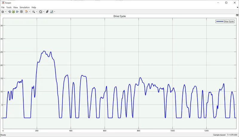
for UDDS drive cycle

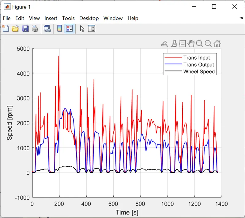
Time trace for engine, transmission input, transmission output and wheel speed:

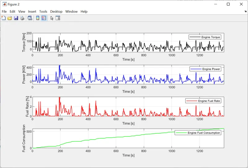
engine torque, engine power, fuel rate and fuel consumption:

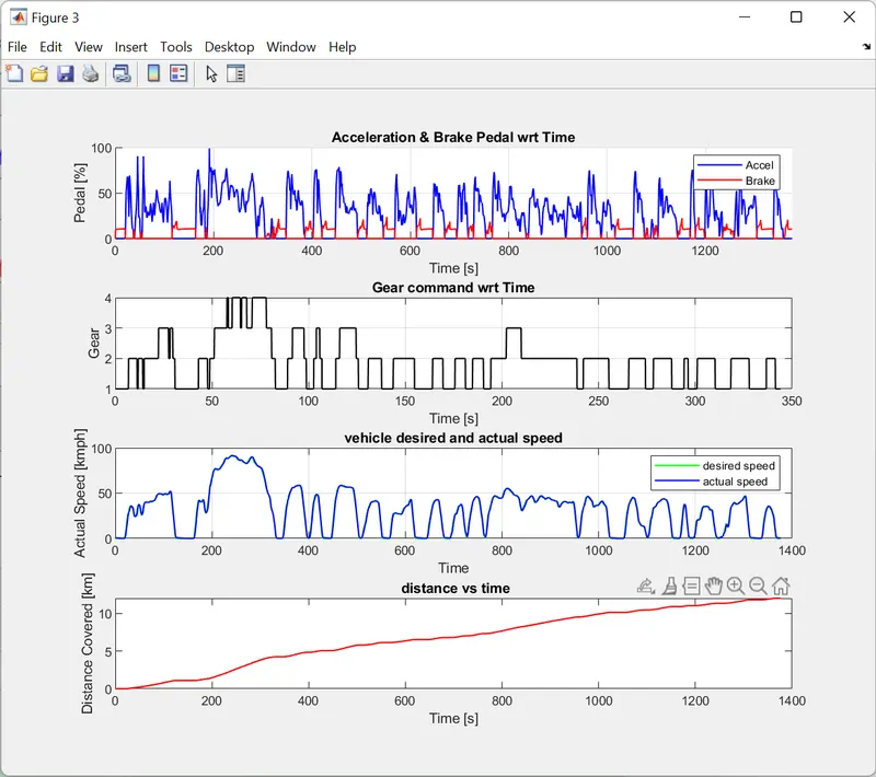
accelerator and brake pedal, gear command, vehicle desired and actual speed, vehicle distance:

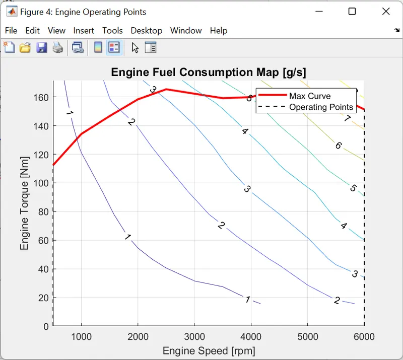
engine operating points on the engine fuel map:

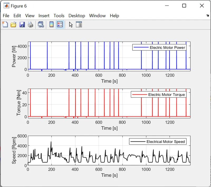
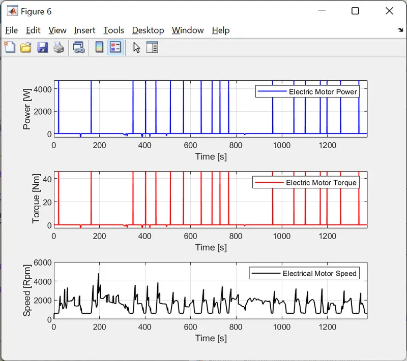
motor speed, torque, motor input power:

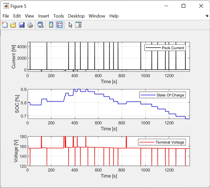
Plot pack voltage, current and SoC:

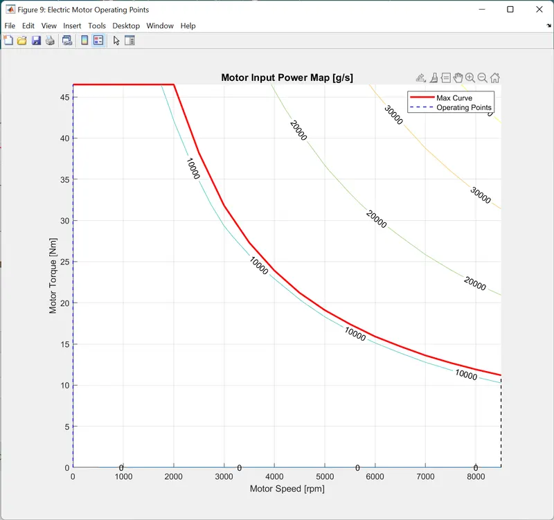
motor operating points on the motor input power map, with the motor max motoring and generating torque curves:

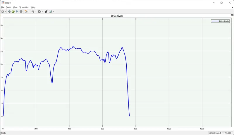
HWFET Drive Cycle:

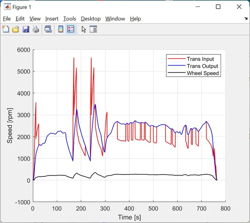
Time trace for engine, transmission input, transmission output and wheel speed:

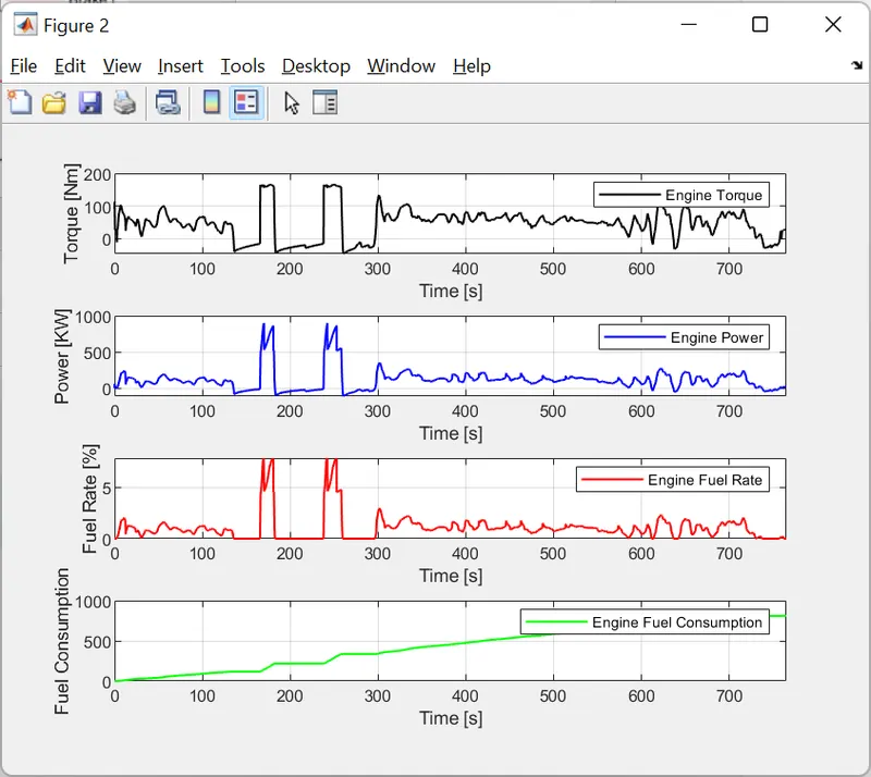
engine torque, engine power, fuel rate and fuel consumption:

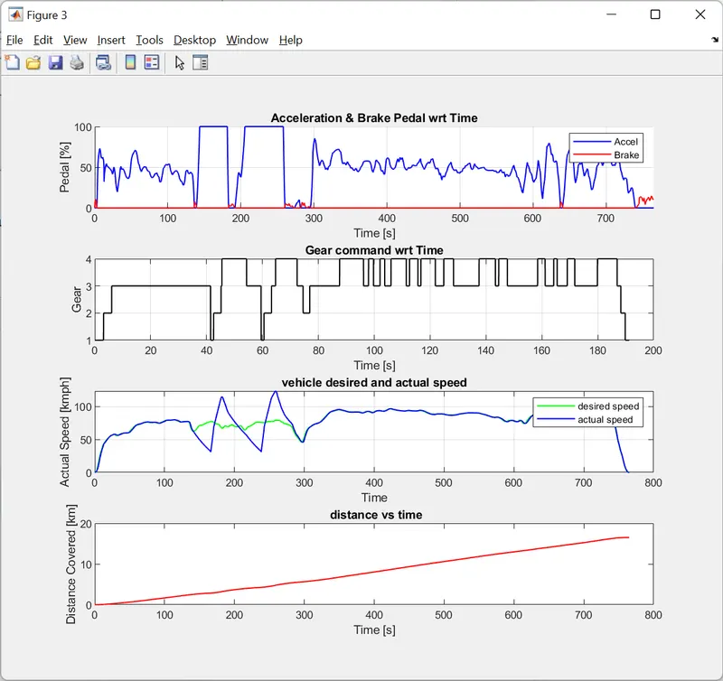
accelerator and brake pedal, gear command, vehicle desired and actual speed, vehicle distance:

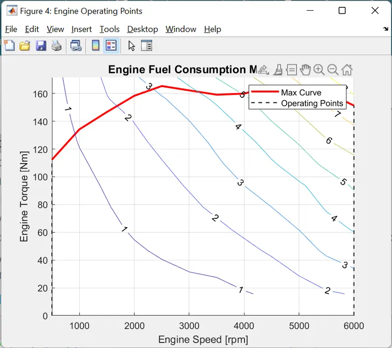
engine operating points on the engine fuel map:

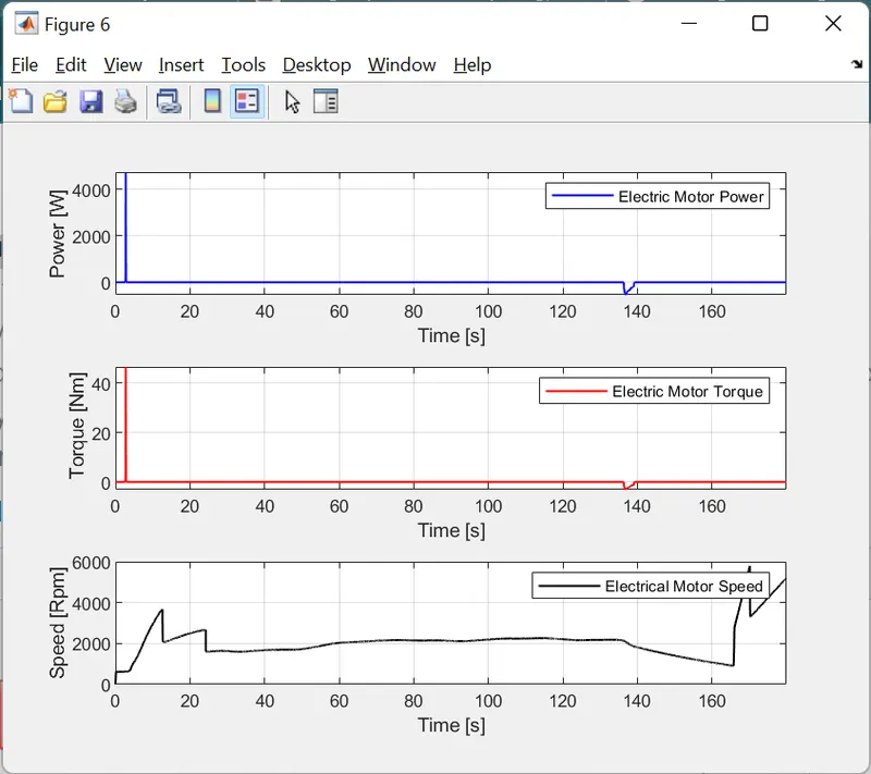
motor speed, torque, motor input power:

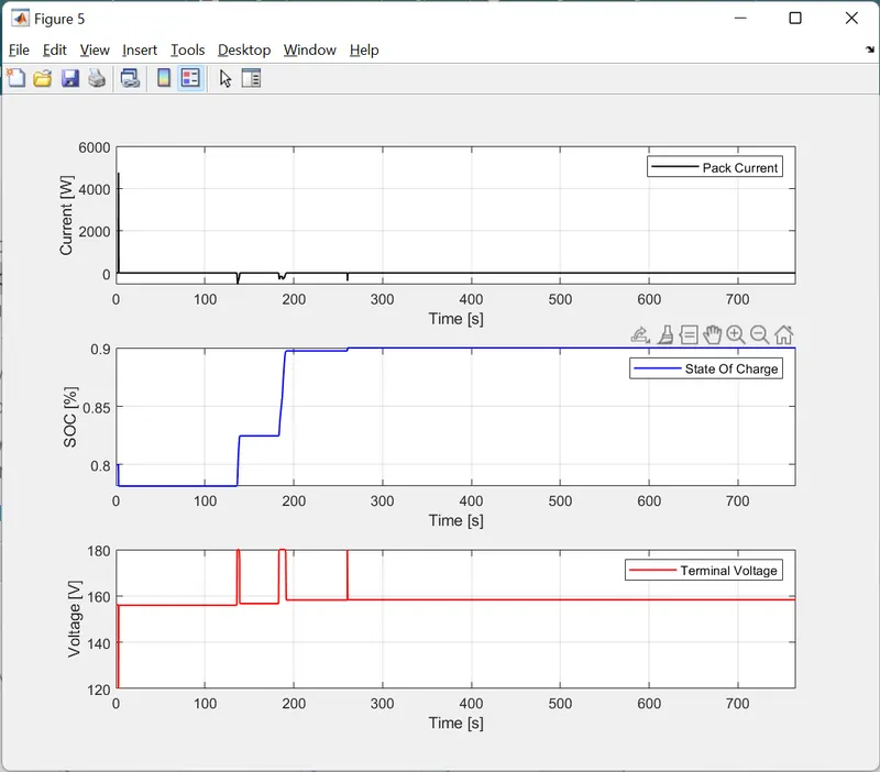
pack voltage, current and SoC:

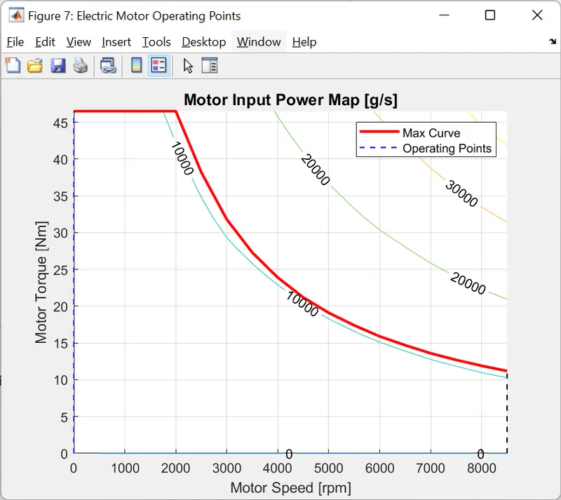
motor operating points on the motor input power map, with the motor max motoring and generating torque curves:

OBSERVATIONS:

fuel economy numbers (kmpl):

For P1 hybrid:

UDDS -> 14.8506 km/litre

HWFET -> 17.6587 km/litre

The fuel economy numbers shows that highway fuel economy is higer than the city fuel economy. Form the graph of acceleration and brake pedal it is clearly observed that there is a lot more braking and idling in UDDS than in the HWFET. Hence highway fuel economy , maximum and mean speeds are higher in HWFET. Also, the fuel consumption and fuel rate are higher in HWFET due to higher maximum and mean speeds and lesser disruptions.

For conventional vehicle:

UDDS -> 13.63 km/litre

HWFET -> 16.3072 km/litre

The fuel economy numbers for P1 hybrid are slightly higher when compared to conventional vehicle.

Power consumption and Engine torque:

Power consumption and Engine torque are more in the UDDS compared to HWFET cycle because it has too many starts and stops compared to
HWFET. More power is required when starting from rest and more torque is required to overcome static friction.

Accelerator, brake pedal and gear shifting:
For UDDS, the accelerator and the brake pedal have more fluctuations due to frequent starts and stops. But in HWFET, the brake pedal fluctuations are almost near to the zero line as there are no frequent stops or disruptions.
UDDS cycle mostly runs on 1st, 2nd gears, and 3rd and 4th are rarely used as it is not possible to achieve high speeds in city traffic. In the HWFET cycle, the vehicle mostly runs on 3rd, 4th gears as it will be moving at high speeds. 1st, 2nd gears are used rarely and only when braking is required.
vehicle speeds(maximum and mean speeds) are higher in HWFET compared to UDDS. UDDS has more fluctuations in the speed due to frequent braking.
The distance travelled in the given time will be high in HWFET than UDDS in a given time as there are no disruptions like frequient braking due to city traffic.

SOC , Pack Voltage, Pack Current:

The pack voltage and current shows more fluctuations in UDDS as compared to HWFET cycle due to frequent starts and stops throughout the drive cycle and the battery has to provide the energgy everytime when the car is starts from the stop.

SOC decreases in the UDDS cycle wrt time but increases in HWFET cycle. This is because in UDDS we have frequent start and stops and battery has to provide the energy has evertytime when the caris starting from the idle position and the SOC decreases but in HWFET cycle The vehicle will be moving continuously without braking frequently and the alternator is used to transfer some engine power to the battery through motor hence SOC increases in the HWFET cycle.

Project 2

Ship work like this
in your own course.

Talk to a career counsellor

Ship work like thisin your own course.

Talk to a career counsellor

Ship work like this
in your own course.