Project 1
% Initialization File
% Initialization file for loading the variables for the Conventional vehicle simulation model
% Vehicle Parameters
M = 1500; % Vehicle weight [kg]
Cr = 0.015; % Rolling resistance coefficient
Rw = 0.35; % Rolling radius [m]
Cd = 0.33; % Drag coefficient
Af = 2; % Frontal area [m2]
rhoa = 1.225; % Air density [kg/m3]
Vwind = 0; % Wind velocity [kmph]
g = 9.81; % Gravitational acceleration [m/s2]
theta = 0; % Slope [deg]
myu_road_tire = 1; % Coefficient of friction between tire - road interface
Tm = 150 ; %Motor torque
efft = 0.8; %Transmission efficiency
ratio = 2.45; %Total ratio
% Vehicle top speed
Vveh = sqrt((efft*ratio/Rw*Tm - Cr*M*g)*2/rhoa/Af/Cd);
Vveh_kmph = 18/5*Vveh;
%% Power for top speed
Fload = 0.5*rhoa*Cd*Af*(Vveh+Vwind)^2 + Cr*M*g*cosd(theta) + M*g*sind(theta); %Road load in N
Pload = Fload*Vveh/1000; % Road load power in KW
%%% Powertrain speed
omegam = ratio*Vveh/Rw;
omega_rmp = omegam*30/pi;
%% Powertrain Parameters
FDR = 3.73; % Final Drive Ratio / Diff Ratio
DiffEff = 0.99; % Differential efficiency (assumed independent of operating conditions)
NumGear = 4; % Number of gears in transmission
TransGear = [1:NumGear]; % Transmission Gears
TransRatio = [3.06, 1.62, 1, 0.7]; % Corresponding Transmission ratios
TransEff = 0.90; % Transmission efficiency (assumed independent of operating conditions)
TC_SR = [0, .5, .6, .7, .8, .87, .92, .94, .96, .97, 1]; % Torque Converter Speed Ratio (Matlab default) -> TurbSpd/PumpSpd
TC_TR = [2.232, 1.5462, 1.4058, 1.2746, 1.1528, 1.0732, 1.0192, 1, 1, 1, 1]; % Torque Converter Torque Ratio (Matlab default) -> TurbTrq/PumpTrq
TC_Cf = 1e-4 * [.72558, .66322, .63463, .59042, .51331, .4144, .29287, .22444, .12186, .04386, 0]; % Torque Converter Capacity Factor (Matlab default) -> PumpTrq/PumpSpd^2 [Nm/rpm^2]
load Vehicle_Data/Engine_data_1_9L_Saturn_95kW
load Vehicle_Data/Trans_Shift_map
%% Driver Parameters
Kp = 10; % P gain for driver PI model
Ki = 1; % I gain for driver PI model
Drive_Cycle_Select = 1; % Drive cycle selection
% Drive cycle values in m/s
if Drive_Cycle_Select == 1
load DriveCycles/UDDS;
elseif Drive_Cycle_Select == 2
load DriveCycles/HWFET;
elseif Drive_Cycle_Select == 3
load DriveCycles/FTP;
elseif Drive_Cycle_Select == 4
load DriveCycles/US06;
elseif Drive_Cycle_Select == 5
load DriveCycles/NEDC;
elseif Drive_Cycle_Select == 6
load DriveCycles/WLTP;
end
time_end = cyc_time(end);
vel_end = cyc_vel(end);
Vehicle Model
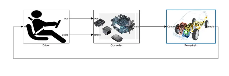
Driver Model:
A driver model is a mathematical model which replicates the functionality of a driver( controlling , monitoring and stabilizing a vehicle )during various maneuvers . In this case, it a PI controller is a basic PI controller that generates accelerator and brake pedal outputs to match the desired and actual vehicle speeds.
Controller Model:
The Controller block represents the electronic controls units. It is based on the driver inputs, it generates desired engine torque, desired transmission gear and desired brake torque. These inputs are fed to the ‘Powertrain’ block which represents the drivetrain of the vehicle.
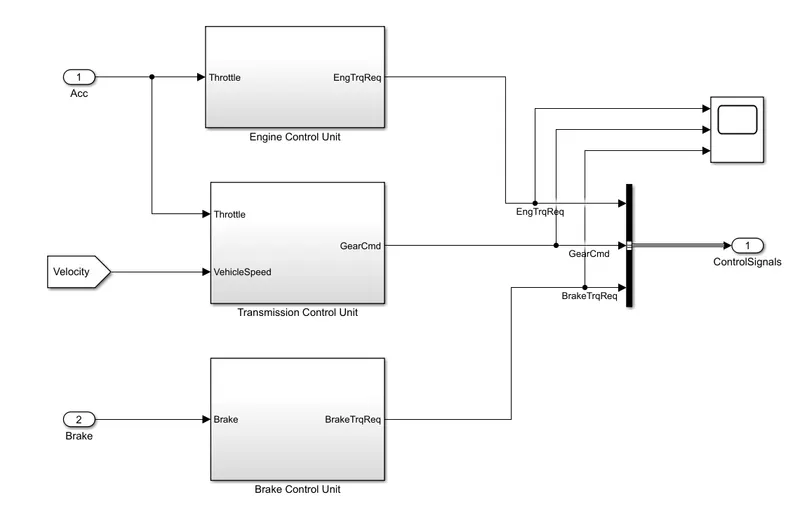
Engine Control Unit:
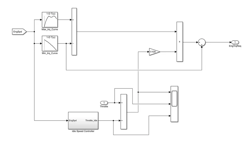
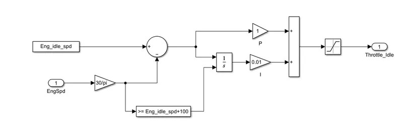
Idle Speed Controller
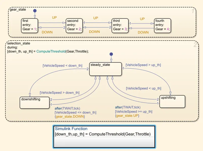
Transmission Control Unit
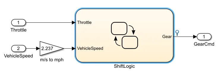
Shift Logic
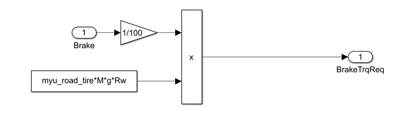
Brake Control Unit
Powertrain Unit
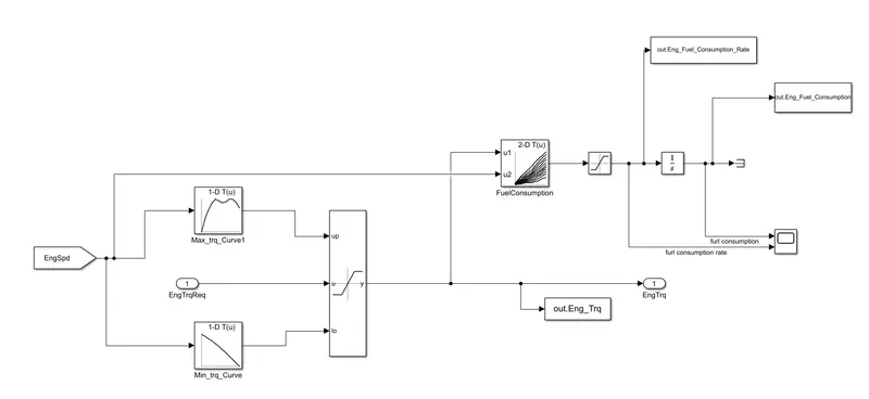
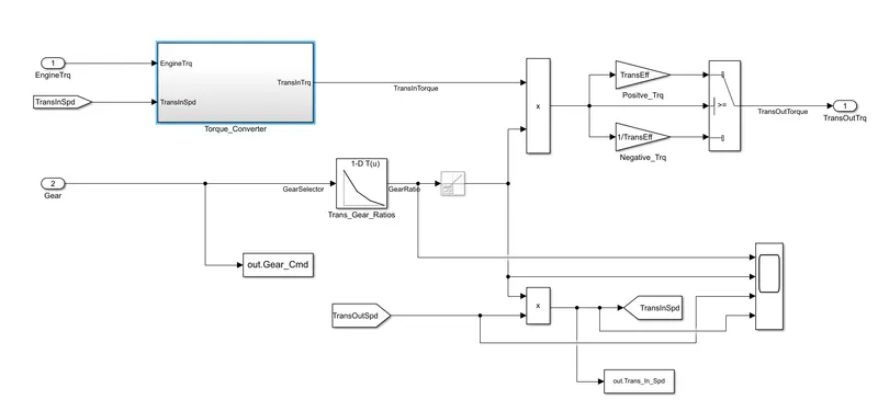
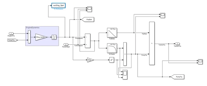
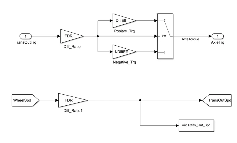
Objective of powertrain modeling is to analyse the powertrain for various drive cycles & vehicle target performances to decide, Traction Motor sizing (Motor nominal & peak torque and current, RPM, Operating Points at various loads & speeds, motor Power, motor efficiency & motor regeneration energy possibilities etc.)
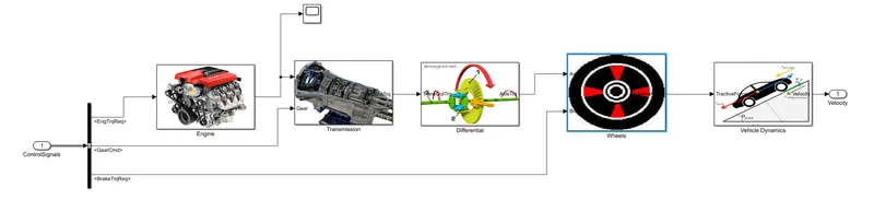
Engine
Transmission
Torque Converter
Differential
Wheels
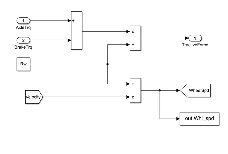
Vehicle Dynamics
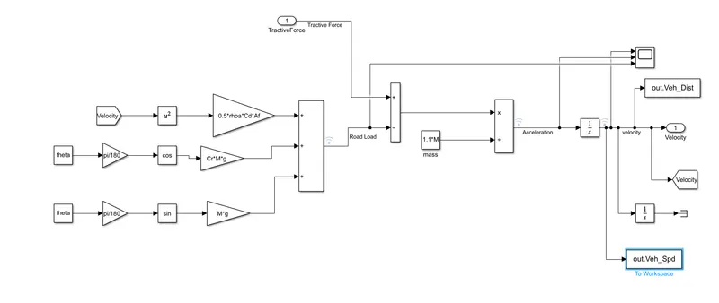
Equations for aerodynamic drag, rolling resistance, and gradient are implemented and added using simulink blocks to get road load.
Road load is subtracted from the tractive force to get the inertia force. Inertia force is then divided by the mass to get the acceleration.
Road load is subtracted from the tractive force to get the inertia force. Inertia force is then divided by the mass to get the acceleration.
Acceleartion is integrated to get speed which is again integrated to get distance travelled.
Speed is used in the closed loop operation.
'To workspace' bloacks are implemented in the models for further calulations and plotting.
RESULTS :
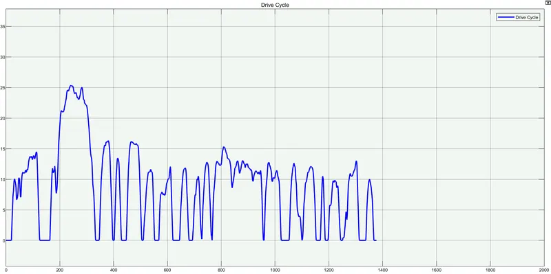
UDDS Cycle
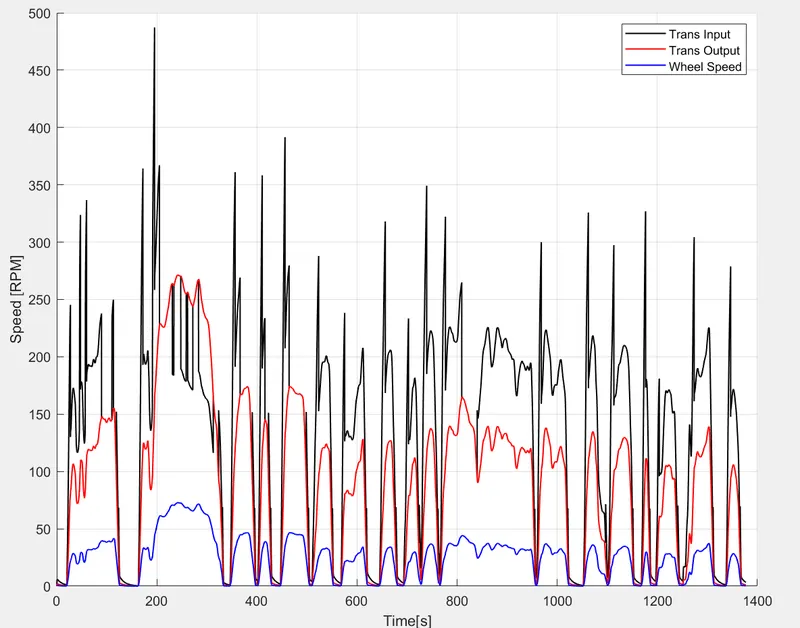
Plotting time trace for engine transmission input & output speed and wheel speed :
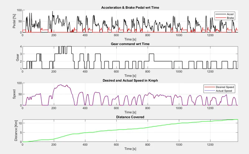
Plotting accelerator and brake pedal, gear command, vehicle desired and actual speed, vehicle distance
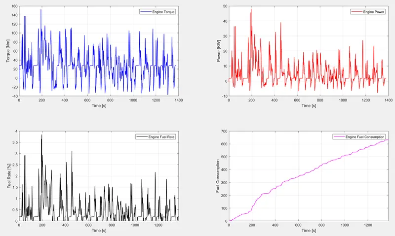
Plotting engine torque, engine power, fuel rate and fuel consumption
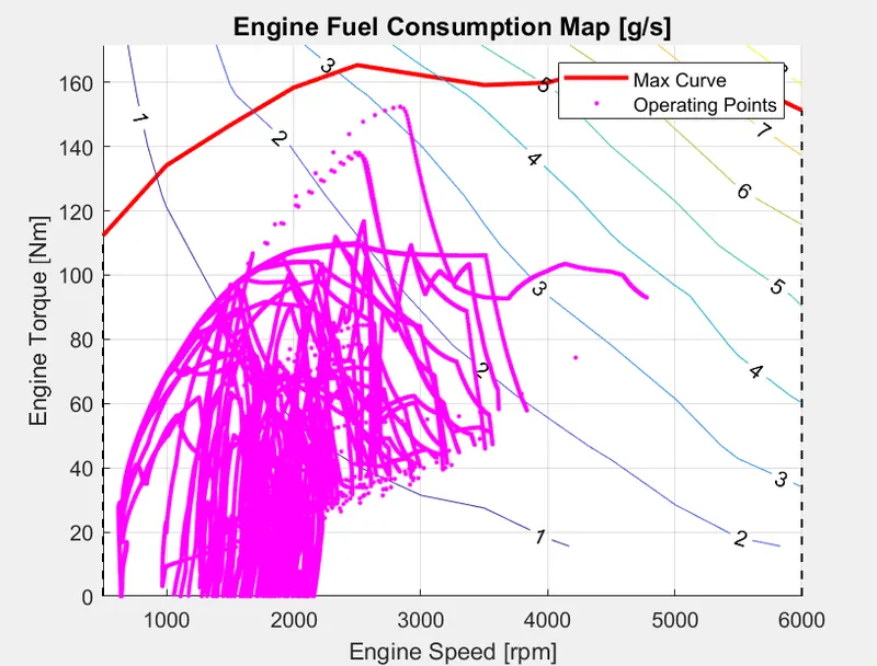
Plotting engine operating points on engine fuel map
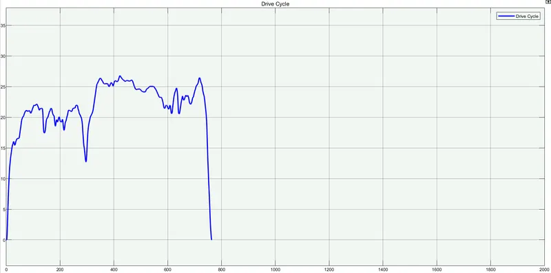
HWFET Cycle:
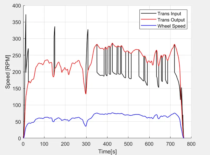
Plotting time trace for engine transmission input & output speed and wheel speed
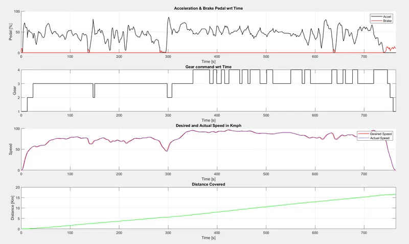
Plotting accelerator and brake pedal, gear command, vehicle desired and actual speed, vehicle distance
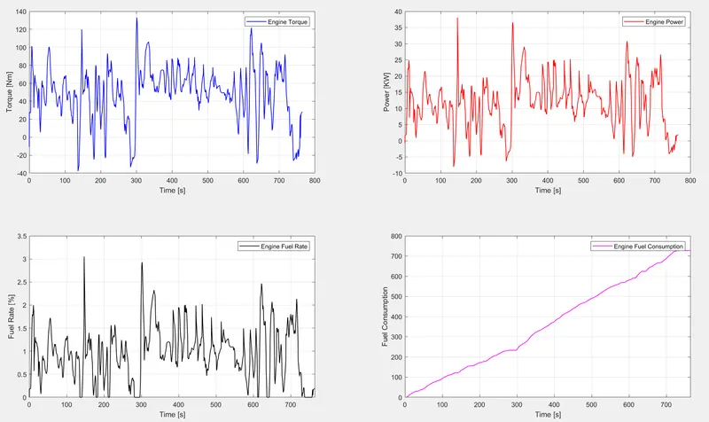
Plotting engine torque, engine power, fuel rate and fuel consumption
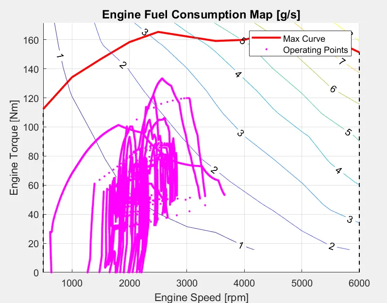
Plotting engine operating points on engine fuel map
Observations:
fuel economy numbers (kmpl) for UDDS and HWFET cycle :
UDDS -> 13.63 km/litre
HWFET -> 16.3072 km/litre
The fuel economy numbers shows that highway fuel economy is higer than the city fuel economy. Form the graph of acceleration and brake pedal it is clearly observed that there is a lot more braking and idling in UDDS than in the HWFET. Hence highway fuel economy , maximum and mean speeds are higher in HWFET. Also, the fuel consumption and fuel rate are higher in HWFET due to higher maximum and mean speeds and lesser disruptions.
Power consumption and Engine torque:
Power consumption and Engine torque are more in the UDDS compared to HWFET cycle because it has too many starts and stops compared to
HWFET. More power is required when starting from rest and more torque is required to overcome static friction.
HWFET. More power is required when starting from rest and more torque is required to overcome static friction.
Accelerator, brake pedal and gear shifting:
For UDDS, the accelerator and the brake pedal have more fluctuations due to frequent starts and stops. But in HWFET, the brake pedal fluctuations are almost near to the zero line as there are no frequent stops or disruptions.
UDDS cycle mostly runs on 1st, 2nd gears, and 3rd and 4th are rarely used as it is not possible to achieve high speeds in city traffic. In the HWFET cycle, the vehicle mostly runs on 3rd, 4th gears as it will be moving at high speeds. 1st, 2nd gears are used rarely and only when braking is required.
vehicle speeds(maximum and mean speeds) are higher in HWFET compared to UDDS. UDDS has more fluctuations in the speed due to frequent braking.
The distance travelled in the given time will be high in HWFET than UDDS in a given time as there are no disruptions like frequient braking due to city traffic.
For UDDS, the accelerator and the brake pedal have more fluctuations due to frequent starts and stops. But in HWFET, the brake pedal fluctuations are almost near to the zero line as there are no frequent stops or disruptions.
UDDS cycle mostly runs on 1st, 2nd gears, and 3rd and 4th are rarely used as it is not possible to achieve high speeds in city traffic. In the HWFET cycle, the vehicle mostly runs on 3rd, 4th gears as it will be moving at high speeds. 1st, 2nd gears are used rarely and only when braking is required.
vehicle speeds(maximum and mean speeds) are higher in HWFET compared to UDDS. UDDS has more fluctuations in the speed due to frequent braking.
The distance travelled in the given time will be high in HWFET than UDDS in a given time as there are no disruptions like frequient braking due to city traffic.