Time = out.tout;
Acceleration_Pdl = out.Acceleration_Pdl; % Accelerator
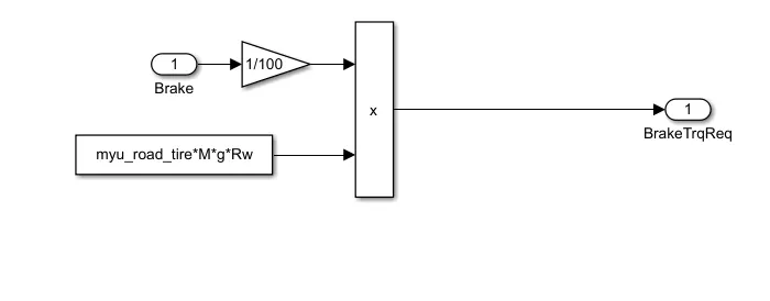
Brake_Pdl = out.Brake_Pdl; % Brake
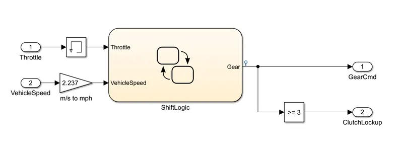
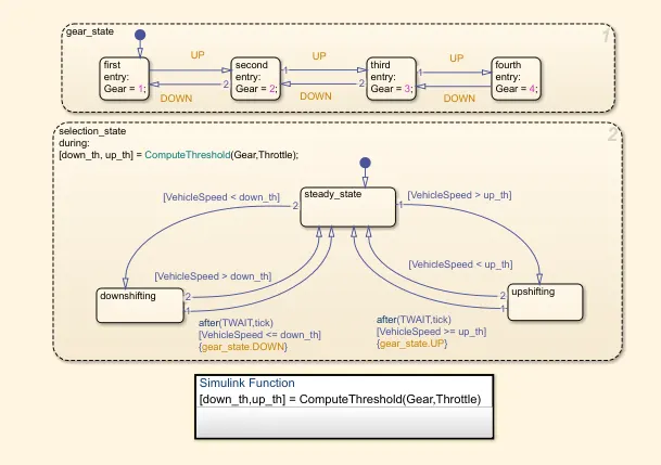
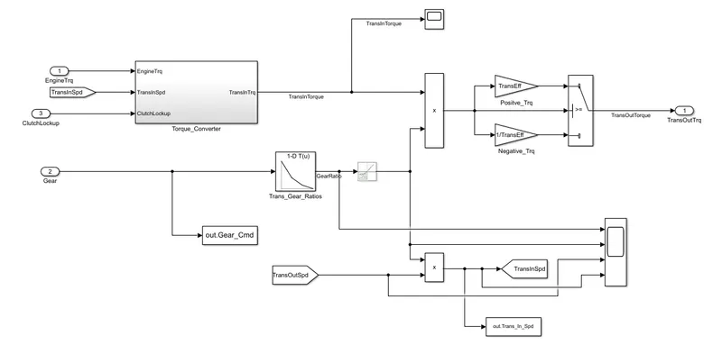
Gear = out.Gear_CMD; % Transmission
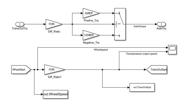
Transmission_In_Spd = out.Trans_In_Spd*30/pi; % Transmission input speed
Transmission_Out_Spd = out.TransOutSpd*30/pi;% Transmission output speed
Engine_Torque = out.Eng_Trq; % Engine brake torque
Engine_Speed = out.Eng_Spd*30/pi; % Engine speed
Engine_Fuel_Consumption = out.Eng_Fuel_Consumption; % Engine fuel consumption
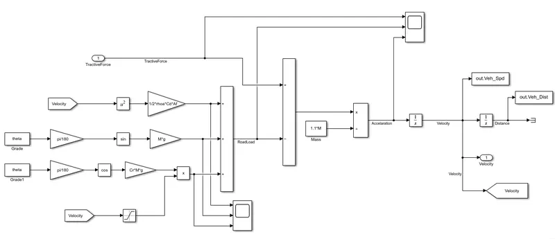
Vehicle_Dist = out.Veh_Dist/1000; % Distance traveled by vehicle
Vehicle_Speed = out.Veh_Spd*18/5; % Vehicle speed
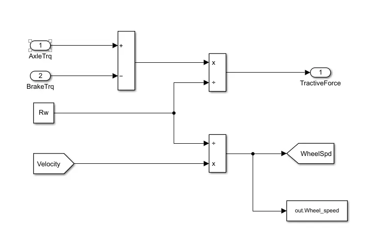
Wheel_Speed = out.WheelSpeed; % Wheel speed
Engine_Fuel_Rate = out.Eng_Fuel_Rate % Engine fuel rate
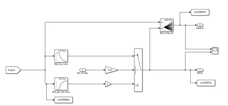
EM_Speed = out.EMSpd*18/5; % Electric Motor Speed
EM_Power = out.EMPwr; % Electric Motor Power
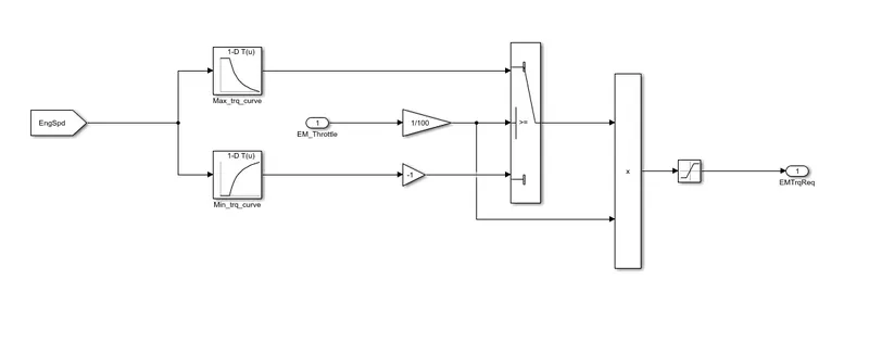
EM_Torque = out.EMTrq; % Electric Motor Torque
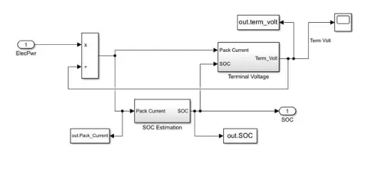
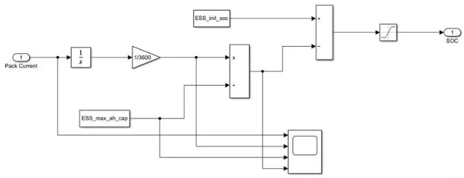
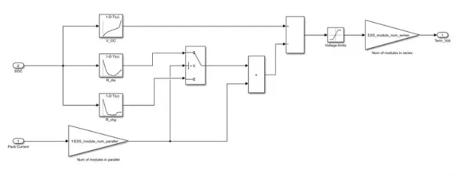
Term_Volt = out.term_volt; % Terminal Voltage of battery
SOC = out.SOC; % State Of Charge
Pack_Current = out.Pack_Current; %Pack current of battery
Eng_Power = Engine_Speed*pi/30*Engine_Torque/1000; % Engine brake power
rho_petrol = 0.7197; % Density of petrol
kmpl = Vehicle_Dist(end)/(Engine_Fuel_Consumption(end)/1000/rho_petrol); % Fuel economy [kmpl]
Eng_spd = Engine_Speed.Data(:,1); % engine speed
Eng_trq = Engine_Torque.Data(:,1); % engine torque
Eng_pwr = Eng_Power.Data(:,1); % engine power
Eng_fuel_rate = Engine_Fuel_Rate.Data(:,1); % engine fuel rate
Eng_fuel_consumption = Engine_Fuel_Consumption.Data(:,1); % engine fuel consumption
EM_speed = EM_Speed.Data(:,1); % motor speed
EM_power = EM_Power.Data(:,1); % Motor Power
EM_torque = EM_Torque.Data(:,1); % Motor Torque
Pack_current = Pack_Current.Data(:,1); %pack current of battery
State_of_charge = SOC.Data(:,1); %state of charge
Term_voltage = Term_Volt.Data(:,1); % terminal Voltage of battery
% Plotting
figure(1)
hold on
grid on
plot(Time, Transmission_In_Spd, 'linewidth', 1, 'Color', 'black');
plot(Time, Transmission_Out_Spd, 'linewidth', 1, 'Color', 'red');
plot(Time, Wheel_Speed, 'linewidth',1, 'color', 'blue')
ylabel('Speed(rpm)')
xlabel('Time(s)')
xlim([0, Time(end)]);
ylim([0, 6000]);
legend('Transmission Input','Transmission Output','Wheel Speed');
%% Plotting
figure(2)
subplot(4,1,1)
plot(Time,Eng_trq,'linewidth',1,'color','black')
xlim([0, Time(end)]);
xlabel('Time(s)')
ylabel('Torque(Nm)')
legend('Engine Torque')
grid on
subplot(4,1,2)
plot(Time,Eng_pwr,'linewidth',1,'color','blue')
xlim([0, Time(end)]);
xlabel('Time(s)')
ylabel('Power(KW)')
legend('Engine Power')
grid on
subplot(4,1,3)
plot(Time,Eng_fuel_rate,'linewidth',1,'color','red')
xlim([0, Time(end)]);
xlabel('Time(s)')
ylabel('Fuel Rate(%)')
legend('Engine Fuel Rate')
grid on
subplot(4,1,4)
plot(Time,Eng_fuel_consumption,'linewidth',1,'color','green')
xlim([0, Time(end)]);
xlabel('Time(s)')
ylabel('Fuel Consumption')
legend('Engine Fuel Consumption')
grid on
% Plotting
figure(3)
plot(Eng_fuel_consumption,Eng_fuel_rate,'color','r')
xlabel('Fuel consumption')
ylabel('Fuel Rate(%)')
title('Fuel economy Vs Fuel Consumption')
grid on
% Potting
figure(4)
subplot(2,1,1)
hold on
plot(Time, Acceleration_Pdl, 'linewidth', 1, 'Color', 'black');
plot(Time, Brake_Pdl, 'linewidth', 1, 'Color', 'red');
ylabel('Pedal (%)')
xlabel('Time (s)');
xlim([0, Time(end)]);
grid on
legend('Acceleraton','Brake');
title('Acceleration & Brake Pedal wrt Time')
subplot(2,1,2)
plot(Time, Gear, 'linewidth', 1, 'Color', 'black');
xlim([0, Time(end)]);
xlabel('Time(s)');
ylabel('Gear');
grid on
title('Gear command wrt Time')
% Plotting
figure(5)
subplot(2,1,1)
plot(Veh_spd, Gear, 'linewidth', 1, 'Color', 'black');
xlabel('Speed(rpm)');
ylabel('Gear');
grid on
title('Gear command wrt vehicle speed')
subplot(2,1,2)
plot(Veh_dist, Gear, 'linewidth', 1, 'Color', 'red');
xlabel('Distance(kmpl)');
ylabel('Gear');
grid on
title('Gear command wrt Distance')
% Plotting
figure('Name','Engine Operating Points');
hold on
grid on
title('Engine Operating Points','fontsize',12);
p1=plot(Eng_map_spd*30/pi,Eng_max_trq,'linewidth',2,'color','r');
p2=line([Eng_map_spd(end)*30/pi Eng_map_spd(end)*30/pi],[0 Eng_max_trq(end)]);
set(p2,'linewidth',1,'linestyle','--','color','k');
p3=line([Eng_map_spd(1)*30/pi Eng_map_spd(1)*30/pi],[0 Eng_max_trq(1)]);
set(p3,'linewidth',1,'linestyle','--','color','k');
[c,h] = contour(Eng_map_spd'*30/pi,Eng_map_trq,Eng_fuel_map');
clabel(c,h);
xlabel('Engine Speed(rpm)');
ylabel('Engine Torque(Nm)');
title('Engine Fuel Consumption Map(g/s)');
legend([p1 p3],{'Max Curve','Operating Points'});
axis([Eng_map_spd(1)*30/pi Eng_map_spd(end)*30/pi 0 Eng_map_trq(end)]);
% State of Charge
figure(6)
subplot(3,1,1)
plot(Time,Pack_current,'linewidth',1,'color','black')
xlim([0, Time(end)]);
xlabel('Time (s)')
ylabel('Current (W)')
legend('Pack Current')
grid on
subplot(3,1,2)
plot(Time,State_of_charge,'linewidth',1,'color','blue')
xlim([0, Time(end)]);
xlabel('Time (s)')
ylabel('Charging (%)')
legend('State Of Charge')
grid on
subplot(3,1,3)
plot(Time,Term_voltage,'linewidth',1,'color','red')
xlim([0, Time(end)]);
xlabel('Time (s)')
ylabel('Voltage (V)')
legend('Terminal Voltage')
grid on
% Motor Speed
figure(7)
subplot(3,1,1)
plot(Time,EM_power,'linewidth',1,'color','black')
xlim([0, Time(end)]);
xlabel('Time (s)')
ylabel('Power (W)')
legend('Electric Motor Power ')
grid on
subplot(3,1,2)
plot(Time,EM_torque,'linewidth',1,'color','blue')
xlim([0, Time(end)]);
xlabel('Time (s)')
ylabel(' Torque (Nm)')
legend('Electric Motor Torque')
grid on
subplot(3,1,3)
plot(Time,EM_speed,'linewidth',1,'color','red')
xlim([0, Time(end)]);
xlabel('Time (s)')
ylabel('Speed (Rpm)')
legend('Electrical Motor Speed')
grid on
% Plotting
figure('Name','Electric Motor Operating Points');
hold on
grid on
title('Electric Motor Operating Points','fontsize',12);
p1=plot(EM_map_spd*30/pi,EM_max_trq,'linewidth',2,'color','r');
p2=line([EM_map_spd(end)*30/pi EM_map_spd(end)*30/pi],[0 EM_max_trq(end)]);
set(p2,'linewidth',1,'linestyle','--','color','k');
p3=line([EM_map_spd(1)*30/pi EM_map_spd(1)*30/pi],[0 EM_max_trq(1)]);
set(p3,'linewidth',1,'linestyle','--','color','k');
[c,h] = contour(EM_map_spd'*30/pi,EM_map_trq,EM_inpwr_map');
clabel(c,h);
xlabel('Motor Speed (rpm)');
ylabel('Motor Torque (Nm)');
title('Motor Input Power Map [g/s]');
legend([p1 p3],{'Max Curve','Operating Points'});
axis([EM_map_spd(1)*30/pi EM_map_spd(end)*30/pi 0 EM_map_trq(end)]);
Result graph :
UDDS :
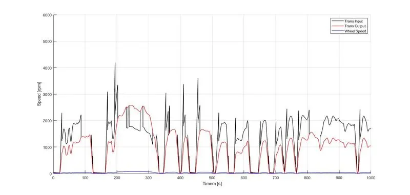
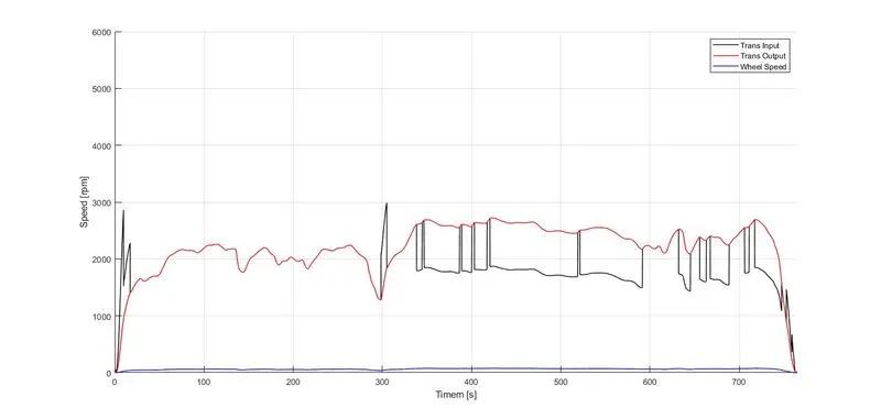
(time trace for engine, transmission input, transmission output and wheel speed on one plot) :
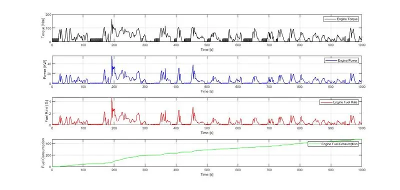
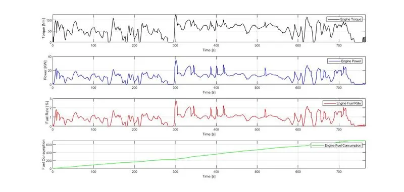
(engine torque, engine power, fuel rate and fuel consumption using subplots) :
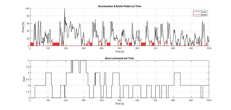
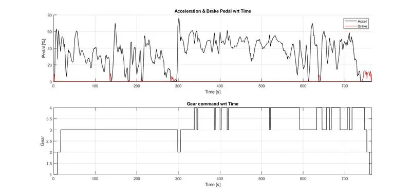
(accelerator and brake pedal, gear command, vehicle desired and actual speed, vehicle distance using subplots) :
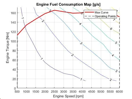
(engine operating points on the engine fuel map) :
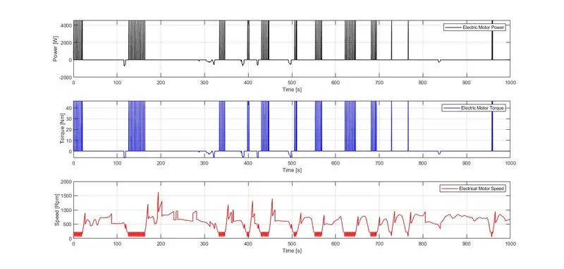
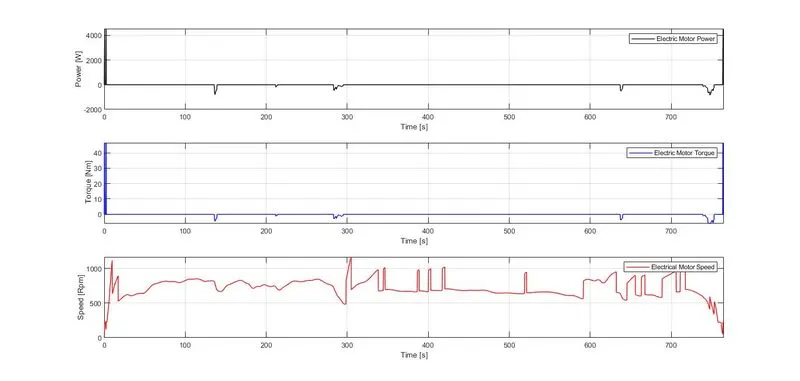
(motor speed, torque, motor input power using subplots) :
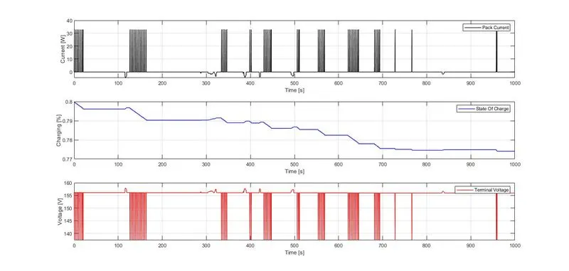
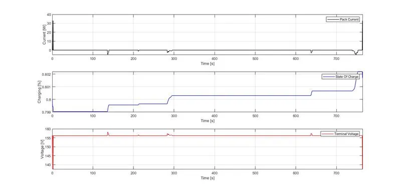
(pack voltage, current and SoC using subplots) :
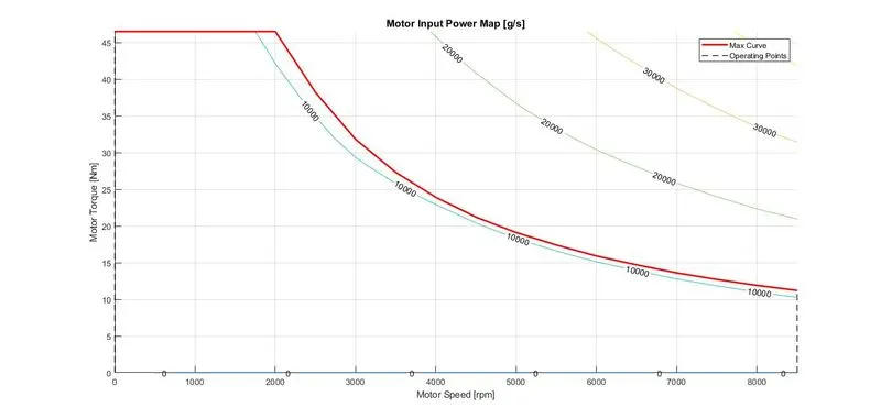
motor operating points on the motor input power map, with the motor max motoring and generating torque curves):
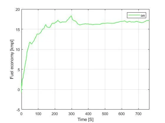
(Fuel economy v/s time) :
HWFET :
(time trace for engine, transmission input, transmission output and wheel speed on one plot) :
(engine torque, engine power, fuel rate and fuel consumption using subplots) :
(accelerator and brake pedal, gear command, vehicle desired and actual speed, vehicle distance using subplots) :
(engine operating points on the engine fuel map) :
(motor speed, torque, motor input power using subplots) :
(pack voltage, current and SoC using subplots) :
(motor operating points on the motor input power map, with the motor max motoring and generating torque curves):
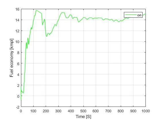
(Fuel economy v/s time) :
-> In this case, we can see that the graph fluctuates more during the UDDS drive cycle than during the HWFET drive cycle. Because HWFET has fewer starts and stops than UDDS, this is the case. Compared to HWFET, UDDS requires more braking.In the UDDS drive cycle, the engine's maximum speed was close to 4200 RPM, but in the HWFET drive cycle, it was 3000 RPM.
-> The car used more electricity in the UDDS driving cycle since it had to make more starts and stops than a HWFET in urban areas. Because the vehicle needs more torque when starting from a standstill to overcome static friction, the engine is higher in the UDDS drive cycle than the HWFET drive cycle. Compared to the UDDS drive cycle, the HWFET drive cycle has a higher fuel rate since it will be moving continuously and require more fuel. Due to the UDDS cycle's frequent starts and stops and the engine's idle position, the fuel efficiency is high in HWFET.
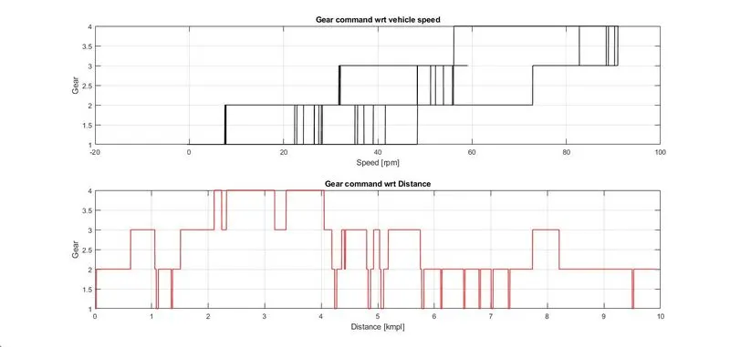
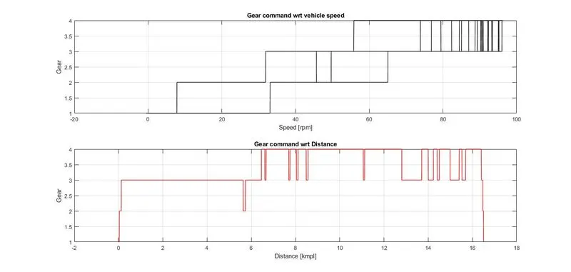
-> Due to the frequent starts and pauses, the accelerator and brake pedals in UDDS experience greater variations. However, because there won't be any frequent stops, the brake pedal fluctuations in HWFET are almost close to the zero line. The first and second gears are used frequently in UDDS cycles, whereas the third and fourth gears are rarely used because the cycle cannot reach high speeds in such traffic. The car runs primarily in third and fourth gears during the HWFET cycle because it will be travelling quickly.