Project 1
Aim :
To compute the fuel economy numbers for the given vehicle (kmpl) on the urban cycle (UDDS) and highway cycle (HWFET). Also, to analyze and understand the vehicle operating
points in terms of engine speed, torque, transmission speeds, pedal positions, gear, distance traveled, etc.
Energy and powertrain efficiency :
In this design, the powertrain must immediately provide the wheel's power demand. In other words, the power from the powertrain determines the power needed at the wheels for performance factors like acceleration, speed, etc. The power comes from the engine through the gearbox because this vehicle's powertrain comprises of an engine that is connected to the wheels through a transmission.
Conventional powertrain efficiency :
The combustion process transforms chemical energy that has been stored into mechanical energy, which the engine uses to produce power. The energy input for this energy conversion process comes from the consumption of fuel, and it is also efficient.
Conventional vehicles :
The wheels of conventional vehicles are propelled by an internal combustion engine that is fuelled by either gasoline or diesel. A fuel and an oxidizer are burned in a combustion chamber to produce expanding gases that press against a piston to produce force and torque. This is how a heat engine works. The fuel's chemical energy is converted into heat in this vehicle's engine and used to create productive work. commonly utilise fossil fuels such as petroleum (petrol and diesel). The 4 stroke reciprocating engine is the most common type of engine utilised in this system. Otto and Diesel cycles are two examples of ideal thermodynamic cycles that can be used to simulate an engine in a cycler. A spark initiated SI engine's cycle mechanism is described by the Otto cycle, an ideal cycle. And the Diesel cycle is the best cycle for describing the operation of a CI engine with compression ignition.
Energy based models- Element models :
There are essentially two different methods for modelling an element's internal physical properties and losses.
- Map based model : Maps that depict the link between input and output, output and losses, etc. are used to simulate many elements.
- Ananlytical model : Physical equations that capture the internal dynamics are used to model elements. These are the two extremes, and the majority of models combine the two, with some dynamics models being analytical and others being based on maps.
In this model We use Forward Model :-
It is often referred to as dynamic modelling. In-depth simulations are performed using dynamic models. This model uses force, torque, and power as inputs and vehicle status variables, such as acceleration and velocity, as outputs. Due to physical casualty, models and simulations are more realistic and suitable for control development. To achieve the desired vehicle state, there is a feedback loop. It is primarily used to replicate a vehicle while it is being driven in order to analyse the dynamic behaviour of the system, which greatly aids in the creation of controls.
Instantaneous fuel consumption is given as :-
m' f = Pe / ηe ⋅ ηt ⋅ QLHV
Where,
mf = mass flow rate in [kg]
pe = Power of engine
pt = power of transmission
nt = efficiency of transmission
ne = efficiency of engine
QLHV = it is th ecalorific value/ lower heating value of fuel.
In this IC engine system, even if there is no power at the wheels, the engine will still use some fuel to maintain rotation and compensate for drag loss. This is known as the idling process. Only when the wheel power is pure power can the aforementioned formula be used. Due to engine drag losses, the engine is either engaged and delivering some engine braking when the wheel power is negative or it is disengaged and idles. Even when the engine is braking, some gasoline may be consumed by the engine because it is idling. In addition to the power needed to turn the wheels, fuel is also needed to create power for the different engine and vehicle accessory loads.
MATLAB :
%%%%%%%%%%%%%%%%%%%%%%%%%%%%%%%%%%%%%%%%%%%%%%%%%%%%%%%
%% Skill-Lync -> Hybrid Drives Development
% Project 1 - Conventional Vehicle Model
% By - Dharmesh Ravindra Bonde
% Description:
%% Initialization File
% Initialization file for loading the variables for the Conventional vehicle simulation model
%% Vehicle Parameters
M = 1500; % Vehicle weight [kg]
Cr = 0.015; % Rolling resistance coefficient
Rw = 0.35; % Rolling radius [m]
Cd = 0.33; % Drag coefficient
Af = 2; % Frontal area [m2]
rhoa = 1.225; % Air density [kg/m3]
Vwind = 0; % Wind velocity [kmph]
g = 9.81; % Gravitational acceleration [m/s2]
theta = 0; % Slope [deg]
myu_road_tire = 1; % Coefficient of friction between tire - road interface
%% Powertrain Parameters
FDR = 3.73; % Final Drive Ratio / Diff Ratio
DiffEff = 0.99; % Differential efficiency (assumed independent of operating conditions)
NumGear = 4; % Number of gears in transmission
TransGear = [1:NumGear]; % Transmission Gears
TransRatio = [3.06, 1.62, 1, 0.7]; % Corresponding Transmission ratios
TransEff = 0.90; % Transmission efficiency (assumed independent of operating conditions)
TC_SR = [0, .5, .6, .7, .8, .87, .92, .94, .96, .97, 1]; % Torque Converter Speed Ratio (Matlab default) -> TurbSpd/PumpSpd
TC_TR = [2.232, 1.5462, 1.4058, 1.2746, 1.1528, 1.0732, 1.0192, 1, 1, 1, 1]; % Torque Converter Torque Ratio (Matlab default) -> TurbTrq/PumpTrq
TC_Cf = 1e-4 * [.72558, .66322, .63463, .59042, .51331, .4144, .29287, .22444, .12186, .04386, 0]; % Torque Converter Capacity Factor (Matlab default) -> PumpTrq/PumpSpd^2 [Nm/rpm^2]
load Vehicle_Data/Engine_data_1_9L_Saturn_95kW
load Vehicle_Data/Trans_Shift_map
%% Driver Parameters
Kp = 10; % P gain for driver PI model
Ki = 1; % I gain for driver PI model
Drive_Cycle_Select = 1; % Drive cycle selection
% Drive cycle values in m/s
if Drive_Cycle_Select == 1
load DriveCycles/UDDS;
elseif Drive_Cycle_Select == 2
load DriveCycles/HWFET;
elseif Drive_Cycle_Select == 3
load DriveCycles/FTP;
elseif Drive_Cycle_Select == 4
load DriveCycles/US06;
elseif Drive_Cycle_Select == 5
load DriveCycles/NEDC;
elseif Drive_Cycle_Select == 6
load DriveCycles/WLTP;
end
time_end = cyc_time(end);
vel_end = cyc_vel(end);
Simulink model :
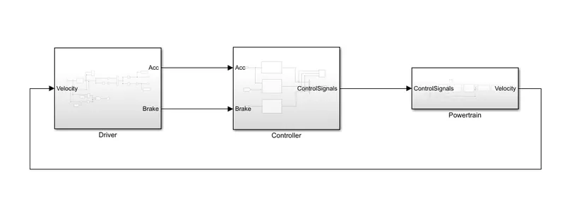
Simulink model of a conventional vehicle
Driver :
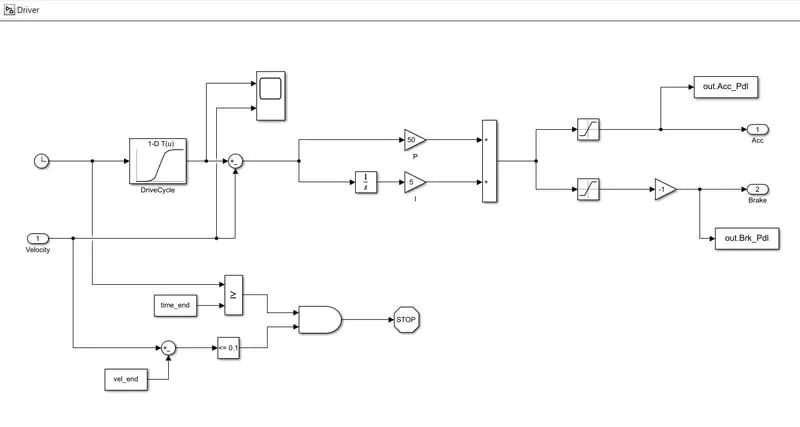
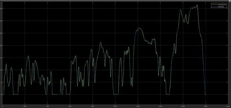
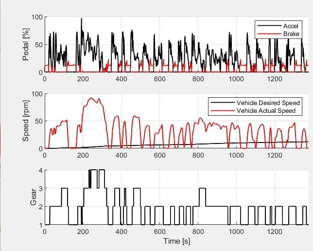
A Driver block, a fundamental PI controller, is used to model it. It creates outputs for the accelerator and brake pedals that correspond to the desired and actual vehicle speeds. We use drive cycles for this since they serve as a basis for uniform assessment and the outcomes of fuel consumption and emissions certification for the vehicle. It is based on time and velocity, after which everything is integrated to produce the accelerator and brake pedals.
Scope :
Controller block :
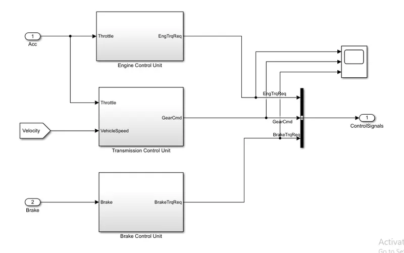
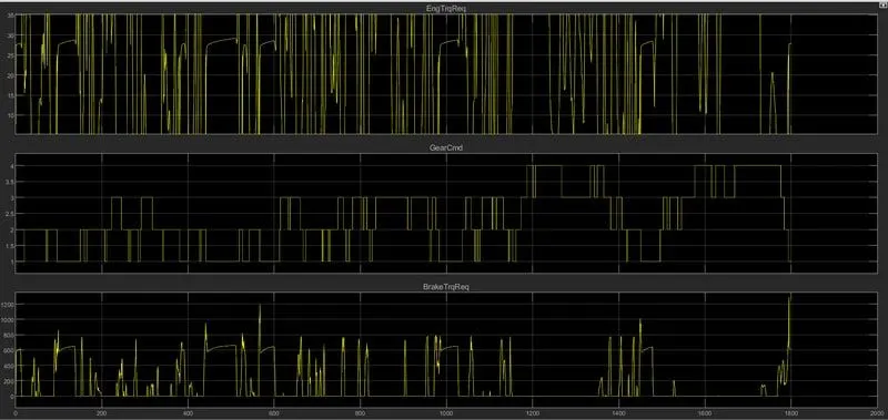
The Controller block, which stands in for the electronic control systems, is the brain of the car. It produces the required engine torque, desired gearbox gear, and desired brake torque dependent on the driver's inputs. These inputs are supplied to the "Powertrain" block, which symbolises the car's drivetrain.
Scope :
Engine control unit :
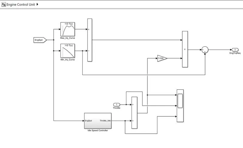
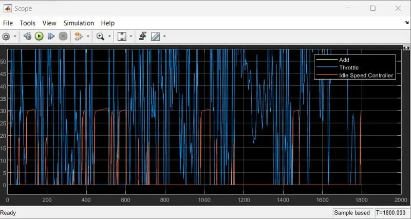
We use an engine control unit in this control model, which provides input for the engine speed by building a look-up table. We feed Maximum torque and map speed into that table, and we also establish a second look-up table in which we input CT torque and map speed, from which it subtracts and multiplies. The engine speed also provides the correct counterspeed to integrate, and as a result, the engine's required torque output is met.
Scope :
Transmission control unit :
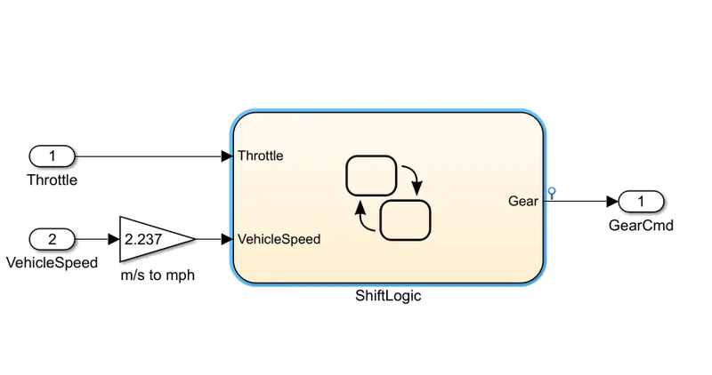
With respect to time, speed, and distance, we build a steady flow variable state in this unit to manage the vehicle's gears in ascending and descending order. and contribute to this steady state is the vehicle's speed, measured in m/s or mph.
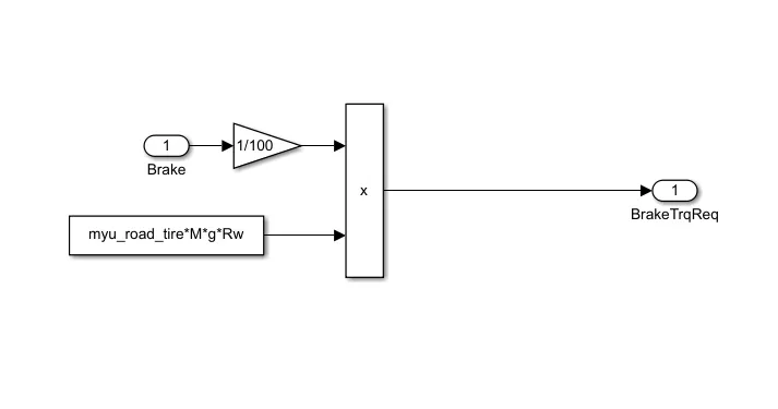
Brake control unit :
This calculation involves the output of all three control signals to the powertrain.
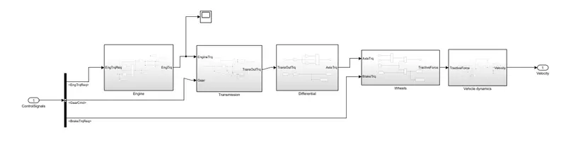
Powertrain Unit :
Every part that transforms the engine's power into movement is included in the powertrain. This covers everything from the engine to the rotating wheels, which includes the driveshaft, differentials, and axles.
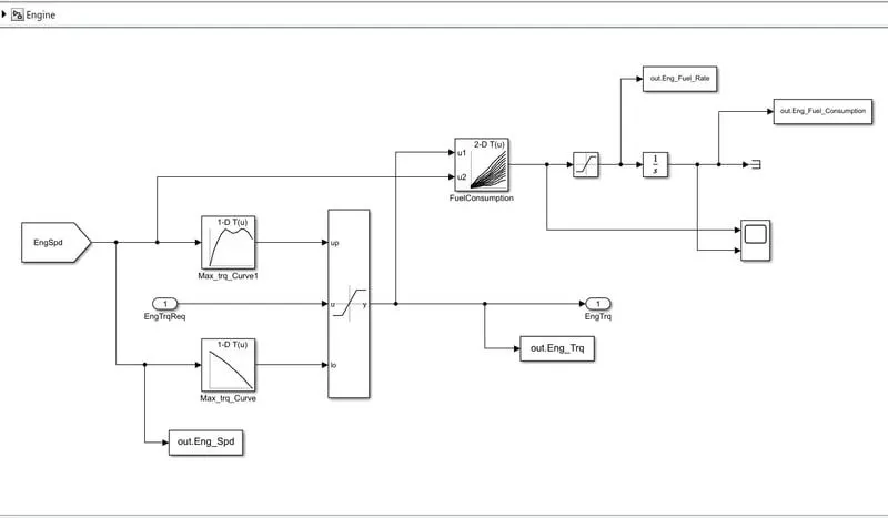
Engine :
To model the engine's fuel consumption in this model, we employed a map-based model. It is based on the controller's maximum torque and minimum torque. and then it takes the speed and torque, goes into saturated output, and then gives the output before saturated torque and speed map produce fuel consumption.
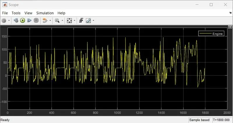
scope :
Transmission :
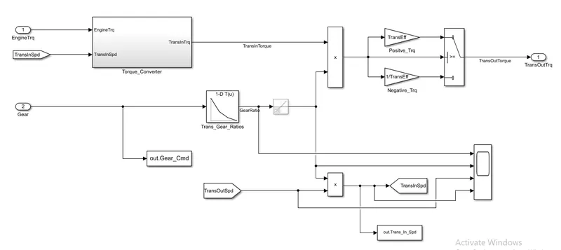
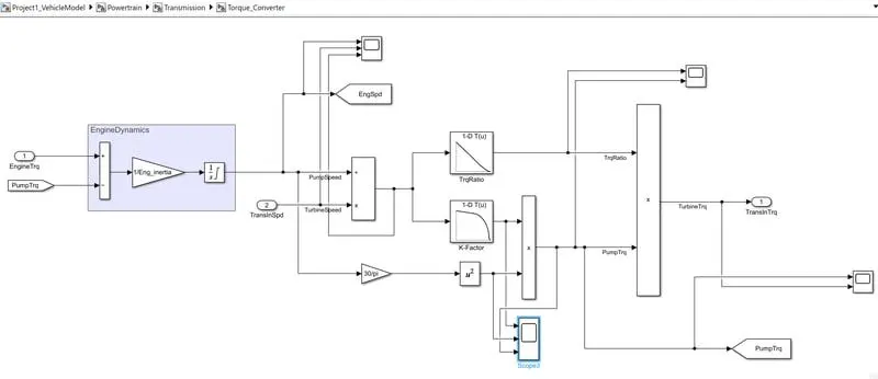
In these models, we use the gear selector from the controllerb for transmission of the gear ratio and the engine torque. The gearbox input speed is determined by multiplying the ratio by the transmission input torque, positive torque, and negative torque, respectively. In this instance, the torque converter is a transmission component that connects the engine to the transmission. It essentially has decoupled engine dynamics.
Torque converter :
Scope :
Differential unit :
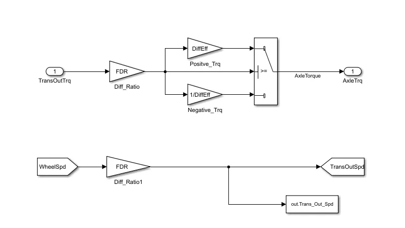
Axle torque is then met after the transmission's output has been multiplied by the input and output torques and passed through the differential ratio. The differential ratio and transmission torque are greater than the axle torque.
Wheel unit :
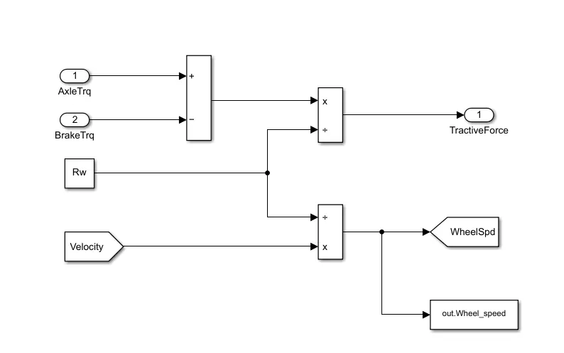
In this model, we take the braking torque from the controller and the axle torque from the differential. Rolling radius and speed are subtracted from and multiplied before we encounter the tractive force from axle and braking torque. and velocity is used to satisfy the wheelspeed.
Vehicle dynamics unit :
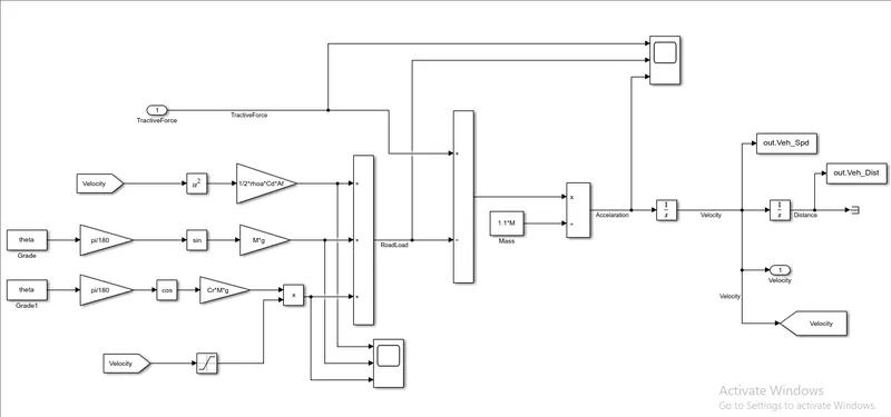
Tractional force and road load are factors in this. Based on tractive force and road load, it determines how fast a vehicle should go.
the dynamic equation for calculating road load is

where,
p = air density [kg/m^3]
A = Frontal area [m^2]
Cd = drag Coefficiend
Vveh = velocity of vehicle [m/s^2]
Vwind = velocity of wind [m/s^2]
Cr = rolling resistance coefficient
M = mass in [Kg]
g = gravity.
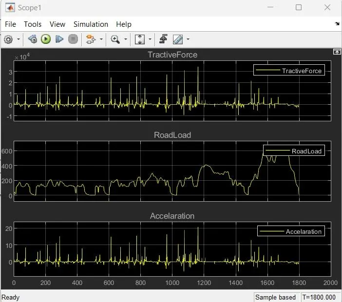
Following calculations and integration, we arrive to the vehicle's acceleration and velocity, which correspond to the vehicle's distance and speed.
Scope :
-> Computing the fuel economyu numbers using UDDS and HWFET cycles:
UDDS Drive cycle:
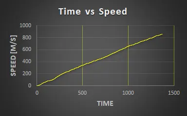
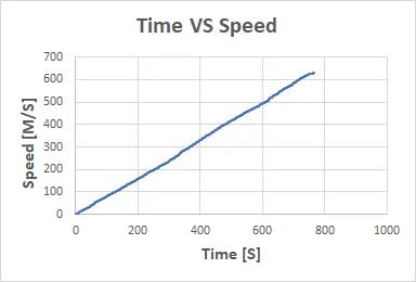
Time VS Speed :
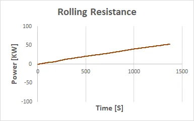
Rolling Resistance :
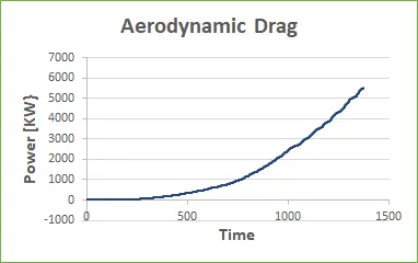
Aerodyanamic drag :
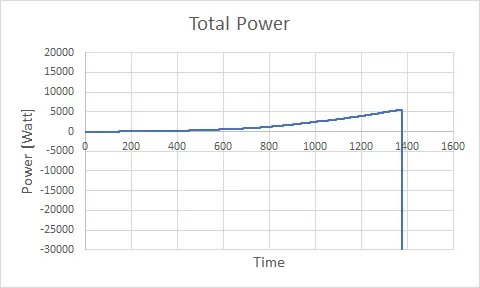
Total power = aerodynamic drag+rolling resistance+inertial resistance
Conclusion:
As rolling resistance, aerodynamic drag, and inertial resistance increase, total power gradually rises.
HWFET Drive Cycle:
Time VS Speed :
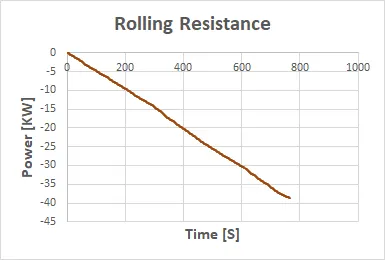
Rolling Resistance :
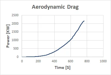
Aerodynamic Drag :
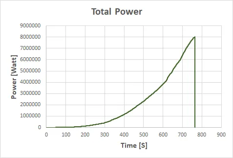
Total Power:- aerodynamic drag+rolling resistance+inertial resistanc`
Conclusion:
As inertial resistance and aerodynamic drag increase, total power gradually rises. However, the decreasing rolling resistance in this drive cycle results in a detrimental impact.
We used the UDDS driving cycle to compare the two cycles. It is preferable to evaluate the fuel usage and pollutant emissions of a vehicle in a consistent manner.
MATLAB script for plotting :
%%%%%%%%%%%%%%%%%%%%%%%%%%%%%%%%%%%%%%%%%%%%%%%%%%%%%%%
%% Skill-Lync -> Hybrid Drives Development
% Project 1 - Conventional Vehicle Model
% By - Dharmesh Ravindra Bonde
% Description:
% The following file is to used with the Initialization file and Simulink
% results for post-processing of the data.
% The file is incomplete, has some examples of how the data is imported
% into a readable format, data analysis and plotting examples.
% Based on the project task, use commands in a similar format as given
% below, to analyse the data and generate required plots.
% You can change variable names if desired
%% Post-Processing File
% File for post-processing the Conventional vehicle simulation model data
%% Renaming variables
Time = out.tout;
Acc_Pdl = out.Acc_Pdl; % Accelerator pedal [%]
Brk_Pdl = out.Brk_Pdl; % Brake pedal [%]
Gear_Cmd = out.Gear_Cmd; % Transmission gear
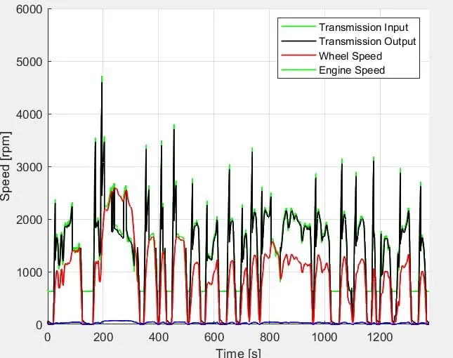
Trans_In_Spd = out.Trans_In_Spd*30/pi; % Transmission input speed [rpm]
Trans_Out_Spd = out.Trans_Out_Spd*30/pi;% Transmission output speed [rpm]
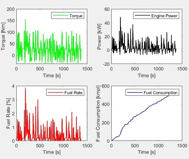
Eng_Trq = out.Eng_Trq; % Engine brake torque [Nm]
Eng_Spd = out.Eng_Spd*30/pi; % Engine speed [rpm]
Eng_Fuel_Consump = out.Eng_Fuel_Consumption; % Engine fuel consumption [g]
Veh_Dist = out.Veh_Dist/1000; % Distance traveled by vehicle [km]
Veh_Spd = out.Veh_Spd*18/5; % Vehicle speed [kmph]
Wheel_Speed = out.wh_speed; % Wheel speed [kmph]
Eng_Fuel_Rate = out.Eng_Fuel_Rate % Engine fuel rate [%]
%% Data Analysis
Eng_Pwr = Eng_Spd*pi/30*Eng_Trq/1000; % Engine brake power [kW]
rho_petrol = 0.7197; % Density of petrol [kg/L]
kmpl = Veh_Dist(end)/(Eng_Fuel_Consump(end)/1000/rho_petrol); % Fuel economy [kmpl]
%% Plotting vehicle characteristics time trace transmission IN/OUT and Wheel Speed
figure(1)
hold on
grid on
plot(Time, Trans_In_Spd, 'linewidth', 1, 'Color', 'black');
plot(Time, Trans_Out_Spd, 'linewidth', 1, 'Color', 'red');
plot(Time, Wheel_Speed, 'linewidth',1, 'color', 'blue')
ylabel('Speed [rpm]')
xlabel('Timem [s]')
xlim([0, Time(end)]);
ylim([0, 6000]);
legend('Trans Input','Trans Output','Wheel Speed');
%% Plotting vehicle characteristics time trace to Engine speed, Engine Torque, Engine Power,
% And Engine fuel rate, Engine fuel consumption
% Data conversion from Double Timeseries
Eng_spd = Eng_Spd.Data(:,1); % engine speed
Eng_trq = Eng_Trq.Data(:,1); % engine torque
Eng_pwr = Eng_Pwr.Data(:,1); % engine power
Eng_fuel_rate = Eng_Fuel_Rate.Data(:,1); % engine fuel rate
Eng_fuel_consumption = Eng_Fuel_Consump.Data(:,1); % engine fuel consumption
Veh_dist = Veh_Dist.Data(:,1); % vehicle distance
Veh_spd = Veh_Spd.Data(:,1); % vehicle speed
% Plotting Engine speed, Engine Torque, Engine Power,Engine fuel rate,Engine fuel consumption wrt Time
figure(2)
subplot(2,2,1)
plot(Time,Eng_trq,'linewidth',1,'color','black')
xlabel('Time [s]')
ylabel('Torque [Nm]')
legend('Engine Torque')
grid on
subplot(2,2,2)
plot(Time,Eng_pwr,'linewidth',1,'color','blue')
xlabel('Time [s]')
ylabel('Power [KW]')
legend('Engine Power')
grid on
subplot(2,2,3)
plot(Time,Eng_fuel_rate,'linewidth',1,'color','red')
xlabel('Time [s]')
ylabel('Fuel Rate [%]')
legend('Engine Fuel Rate')
grid on
subplot(2,2,4)
plot(Time,Eng_fuel_consumption,'linewidth',1,'color','green')
xlabel('Time [s]')
ylabel('Fuel Consumption')
legend('Engine Fuel Consumption')
grid on
% Plotting fuel economy Vs Engine Fuel consumption
figure(3)
plot(Eng_fuel_consumption,Eng_fuel_rate,'color','r')
xlabel('Fuel consumption')
ylabel('Fuel Rate [%]')
title('Fuel economy Vs Fuel Consumption')
grid on
%% Potting Accelerator pedal, Brake pedal and gear command with respect to time
figure(4)
subplot(2,1,1)
hold on
plot(Time, Acc_Pdl, 'linewidth', 1, 'Color', 'black');
plot(Time, Brk_Pdl, 'linewidth', 1, 'Color', 'red');
ylabel('Pedal [%]')
xlabel('Time [s]');
xlim([0, Time(end)]);
grid on
legend('Accel','Brake');
title('Acceleration & Brake Pedal wrt Time')
subplot(2,1,2)
plot(Time, Gear_Cmd, 'linewidth', 1, 'Color', 'black');
xlim([0, Time(end)]);
xlabel('Time [s]');
ylabel('Gear');
grid on
title('Gear command wrt Time')
% Plotting gear command vehicle desired with actual speed
figure(5)
subplot(2,1,1)
plot(Veh_spd, Gear_Cmd, 'linewidth', 1, 'Color', 'black');
xlabel('Speed [rpm]');
ylabel('Gear');
grid on
title('Gear command wrt vehicle speed')
subplot(2,1,2)
plot(Veh_dist, Gear_Cmd, 'linewidth', 1, 'Color', 'red');
xlabel('Distance [kmpl]');
ylabel('Gear');
grid on
title('Gear command wrt Distance')
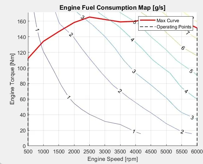
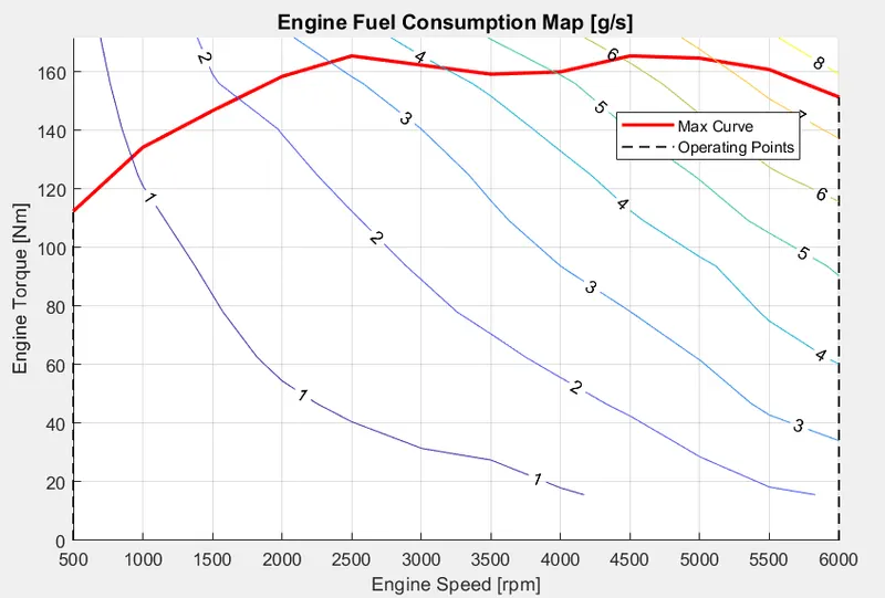
%% Plotting engine operating points on engine fuel map
figure('Name','Engine Operating Points');
hold on
grid on
title('Engine Operating Points','fontsize',12);
p1=plot(Eng_map_spd*30/pi,Eng_max_trq,'linewidth',2,'color','r');
p2=line([Eng_map_spd(end)*30/pi Eng_map_spd(end)*30/pi],[0 Eng_max_trq(end)]);
set(p2,'linewidth',1,'linestyle','--','color','k');
p3=line([Eng_map_spd(1)*30/pi Eng_map_spd(1)*30/pi],[0 Eng_max_trq(1)]);
set(p3,'linewidth',1,'linestyle','--','color','k');
[c,h] = contour(Eng_map_spd'*30/pi,Eng_map_trq,Eng_fuel_map');
clabel(c,h);
xlabel('Engine Speed [rpm]');
ylabel('Engine Torque [Nm]');
title('Engine Fuel Consumption Map [g/s]');
legend([p1 p3],{'Max Curve','Operating Points'});
axis([Eng_map_spd(1)*30/pi Eng_map_spd(end)*30/pi 0 Eng_map_trq(end)]);
Plot results:
UDDS CYCLE :
i) Fuel consumption vs Fuel rate :
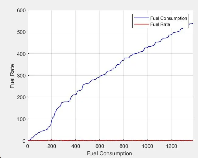
ii) Vehicle characteristics time trace Engine, Transmission input Transmission nout and Wheel speed :
iii) Vehicle characteristics time trace engine torque, Engine power, Fuel rate and fuel consumption :
iv) Vehicle characteristics time trace accelerator and brack pedal, gear command, vehicle desired and actal speed :
v) Engine operating points on engine fuel map :
HWFET CYCLE :
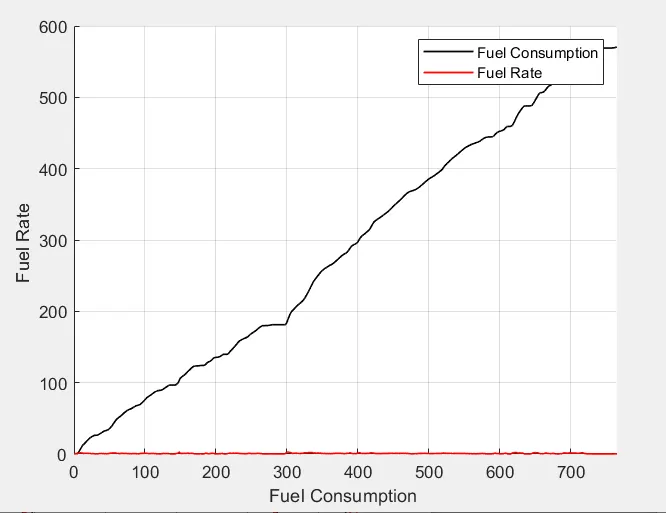
i) Fuel Consumption vs Fuel Rate :
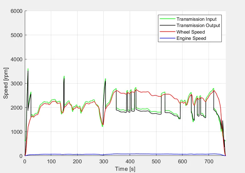
ii) Vehicle characteristics time trace Engine,Transmission Input, Transmission Output and Wheel Speed :
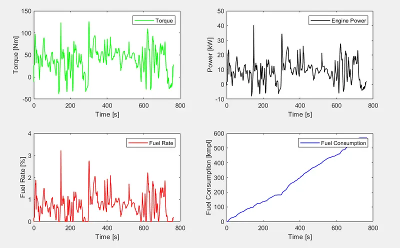
iii) Vehicle characteristics time trace engine torque, engine power, fuel rate and fuel consumption :
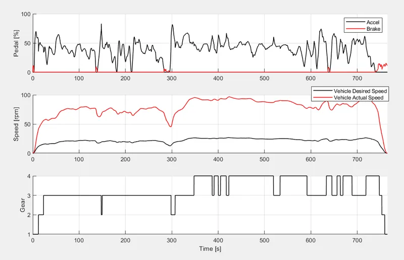
iv) Vehicle characteristics time trace accelerator and brake pedal, gear command, vehicle desired and actual speed :
v) Engine operating points on engine fuel map :
CONCLUSION :
UDDS and HWFET cycle charts were obtained for the Forward energy-based fuel consumption model of a conventional vehicle constructed using MATLAB and SIMULINK.