Project 2

Aim:

To develop a forward energy-based fuel consumption model of a P1 hybrid vehicle and to quantify the improvement in fuel economy numbers, on the UDDS and HWFET cycle as compared to a conventional IC engine vehicle. The model is based on the modifications of a conventional IC engine vehicle.

Objectives:

• Understand the concept of a forward energy-based fuel consumption model of an IC engine vehicle.
• Understand the functioning of various vehicle components such as engine, electric motor, torque converter, transmission system, ECUs, longitudinal dynamics, etc.
• Development of a preliminary Matlab script which will load all the variables required for running the Simulink model.
• Development of the Simulink model for a P1 hybrid vehicle.
• Development of a MATLAB script to do some basic post-process calculations and generate results and plots.
• Analyzing the results.

Theory:

Energy Based Models - Model Structure

There are two basic types of structure for the energy-based models:

-Forward Model: Dynamic simulation of the system

-Backward Model: Quasi-Static simulation of the system

Forward Models

A forward-facing vehicle model features adriver model that provides torque demand in the form of desired ICE torque and brake torque, to meetthe speed trace from a drivecycle. The topology of the forward-facing model that is used in this refer Fig 1. A basic driver model typically uses one or more Proportional-Integral (PI) controllers to achieve the torque demand, with reference to the desired speed trace.

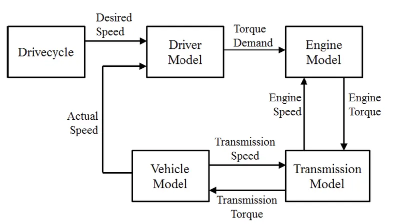
Fig 1

Backward Models

Backward models are calculated in a quasi-static manner. The inputs include vehicle conditions like velocity andacceleration, whereas the output isthe force, torque, and power required at the source, i.e. the engine. They are simple and quick to use, making them ideal for quick computations and comparisons. They lackdynamics, and the method is mostly used to calculate simple fuel consumption and optimize energy management (refer Fig 2).

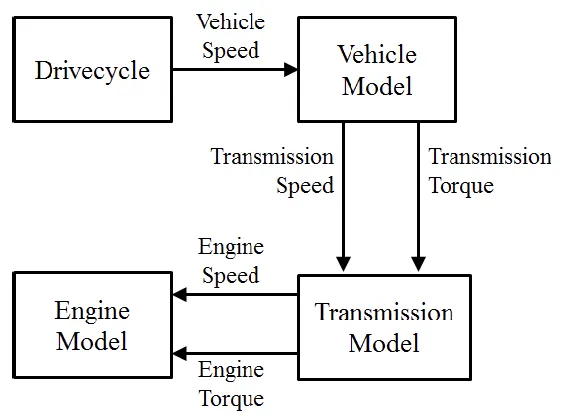
Fig 2

Conventional Vehicle

Conventional vehicles use internal combustion as a heat engine which runs mostly on petroleum-derived products such as diesel or gasoline to drive the wheels. An internal combustion engine (ICE or IC engine) is a heat engine in which the combustion of a fuel occurs with an oxidizer (usually air) in a combustion chamber that is an integral part of the working fluid flow circuit. In an internal combustion engine, the expansion of the high-temperature and high-pressure gases produced by combustion applies direct force to some components of the engine.

P1 Hybrid architecture

A hybrid electric vehicle is a type of hybrid vehicle that combines a conventional internal combustion engine system with an electric propulsion system (hybrid vehicle drivetrain). The presence of the electric powertrain is intended to achieve either better fuel economy than a conventional vehicle or better performance. There is a variety of HEV types and the degree to which each function as an electric vehicle also varies. The most common form of HEV is the hybrid electric car, although hybrid electric trucks (pickups and tractors), buses, boats and aircraft also exist.

The powertrain configuration of the hybrid electric vehicle system has a significant impact on the performance and characteristics of the vehicle, in terms of: integration cost, fuel efficiency, dynamic performance (powertrain torque enhancement) Automotive Original Equipment Manufacturers and automotive Tier 1 system suppliers are currently analyzing and evaluating several major powertrain architectures for hybrid electric vehicles. The electric machine can be positioned, relative to the other powertrain components, in five major points as shown (refer Fig 3)

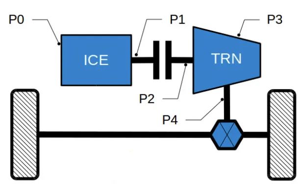
Fig 3

Drive Cycle Development

The "Drive-cycle" basically is the representative of the road. Drive cycles are used to reduce the expense of on-road tests, time of test and fatigue of the test engineer. The whole idea is to bring the road to the test lab (a chassis dynamometer) or to the computer simulation. Data collection from the test road is the most important activity. Testroad (e.g. city, highway, etc.) measured data are the inputs to the 'Drive Cycle' preparation activity.

The procedure involves instrumentation of the test vehicle to collect information while driving on the test road. There are two major types of data to be collected, Driver Behavior data and Vehicle versus Road data. The Vehicle versus Road data is used to prepare the road drive cycle and the Driver Behavior data to prepare the Driver model.

For developing a drive cycle from a real-world driving trip, the data is divided into kinematic sequences. The sequences are classified into distinct clusters. The probability of the occurrence of eachtype of sequence during a certain type of driving trip is calculated. Drive cycles are constructed by randomly selecting sequences based on their probabilities and a cycleis built based on the selection of cycle type, minimum cycle duration, distance, number of stops, average and top speeds, etc.

Energy Based Models - Element Models

To model the internal physical properties of the element and the losses, there are two kinds of approaches: Map based models and Analytical models.

-> Map-based models: Elements are modelled using maps, which characterize the relationship between the input & output and output & losses etc. Map-based models are quite easy to implement in the Simulink workspace.

->Analytical models: Elements are modelled using the physical equations, that represent the internal dynamics. Even though it ispossible to get a better idea of the vehicle system due to the internal dynamics, analytical models are quite difficult to implement practically. Usually, the input work overweighs the result that can be obtained.

Due to the vast number of elements in the P1 hybrid architecture, the map-based model was used to compute the results.

MATLAB Initializing Code:

A MATLAB script “Project2_InitFile.m” is run to load the required variables to the MATLAB base workspace which would be used for the further calculation/processing for the Simulink model. A typical midsize car with a 1.9L engine and a 4-speed automatic transmission coupled with a Honda Insight motor and battery is considered with Data taken from the ADVISOR database developed by NREL, USA. The transmission shift map and controller are taken from Matlab/Simulink example database.

%%%%%%%%%%%%%%%%%%%%%%%%%%%%%%%%%%%%%%%%%%%%%%%%%%%%%%%%%%%%%%%%%%%%%
%% Skill-Lync -> Hybrid Drives Development
% Project 2 - P1 Hybrid Vehicle Model
% By - Aditya Kurup 

% Description:

%% Initialization File
% Initialization file for loading the variables for the Conventional vehicle simulation model

%% Vehicle Parameters
M = 1500;       % Vehicle weight [kg]
Cr = 0.015;     % Rolling resistance coefficient
Rw = 0.35;      % Rolling radius [m]
Cd = 0.33;      % Drag coefficient
Af = 2;         % Frontal area [m2]
rhoa = 1.225;   % Air density [kg/m3]
Vwind = 0;      % Wind velocity [kmph]
g = 9.81;       % Gravitational acceleration [m/s2]
theta = 0;      % Slope [deg]
myu_road_tire = 1; % Coefficient of friction between tire - road interface

%% Powertrain Parameters 
FDR = 3.73;                         % Final Drive Ratio / Diff Ratio
DiffEff = 0.99;                     % Differential efficiency (assumed independent of operating conditions)

NumGear = 4;                        % Number of gears in transmission
TransGear = [1:NumGear];            % Transmission Gears
TransRatio = [3.06, 1.62, 1, 0.7];  % Corresponding Transmission ratios
TransEff = 0.90;                    % Transmission efficiency (assumed independent of operating conditions)

TC_SR = [0, .5, .6, .7, .8, .87, .92, .94, .96, .97, 1];   % Torque Converter Speed Ratio (Matlab default) -> TurbSpd/PumpSpd  
TC_TR = [2.232, 1.5462, 1.4058, 1.2746, 1.1528, 1.0732, 1.0192, 1, 1, 1, 1];   % Torque Converter Torque Ratio (Matlab default) -> TurbTrq/PumpTrq
TC_Cf = 1e-4 * [.72558, .66322, .63463, .59042, .51331, .4144, .29287, .22444, .12186, .04386, 0]; % Torque Converter Capacity Factor (Matlab default) -> PumpTrq/PumpSpd^2 [Nm/rpm^2]

load Vehicle_Data/Engine_data_1_9L_Saturn_95kW
load Vehicle_Data/Trans_Shift_map
load Vehicle_Data/EM_Honda_Insight_10kW
load Vehicle_Data/ESS_NiMH6


ESS_init_soc = 0.8;
ESS_soc_max = 0.9;
ESS_soc_min = 0.6;


%% Driver Parameters
Kp = 10;                    % P gain for driver PI model
Ki = 1;                     % I gain for driver PI model
Drive_Cycle_Select = 1;     % Drive cycle selection

%% Inputting the desired DriveCycle
%Drive_Cycle_Select = input(sprintf('Select a Drive Cycle: n 1. UDDS n 2. HWFET n 3. FTP n 4. US06 n 5. NEDC n 6. WLTP n Your selection is: '));
% Drive cycle values in m/s

%Loading Drive Cycle values. Variables: cyc_time, cyc_vel
if Drive_Cycle_Select == 1
    load DriveCycles/UDDS;
    
elseif Drive_Cycle_Select == 2
    load DriveCycles/HWFET;
    
elseif Drive_Cycle_Select == 3
    load DriveCycles/FTP;
    
elseif Drive_Cycle_Select == 4
    load DriveCycles/US06;
    
elseif Drive_Cycle_Select == 5
    load DriveCycles/NEDC;
    
elseif Drive_Cycle_Select == 6
    load DriveCycles/WLTP;
 
end

time_end = cyc_time(end); %Drive cycle end time
vel_end = cyc_vel(end); %Drive cycle end velocity

%% Running Simulink Model 
%sim('Project2_VehicleModel');   % Run Simulink model

The initialization script loads data from the MATLAB file "Engine_data_1_9L_Saturn_95kW" into the base workspace which includes variables such as Engine efficiency map, Engine fuel map, Engine Inertia, Engine map speed, Engine map torque, maximum and minimum Engine torque values, Battery SOC, minimum and maximum permitted SOC and so on. The MATLAB file "Trans_Shift_map" provides the necessary data required for the control logic of the Transmission control unit. This code is designed in such a way that it asks for the drive cycle that needs to be used for the study and the user input decides the desired drive cycle for the study.

Simulink Vehicle Model

The Simulink model can be summed up with the help of three subsystems.

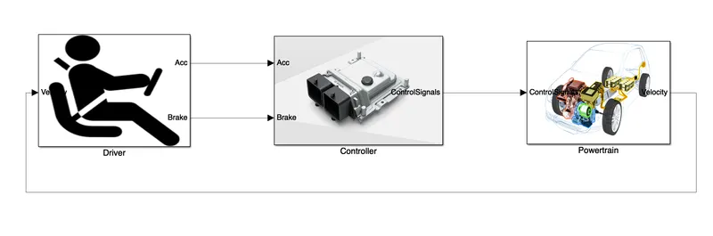
• Driver block
• Controller block
• Power train block

-In brief, the required drive cycle is fed as input to the driver block and it generates the vehicle acceleration and braking percentage requirements whereby simulating a driver input such that the vehicle is following the required drive cycle. This acceleration and brake percentage requirements is fed onto the controller block which then generated the control signals to meet the driver requirements. The generated control signals are then passed onto the Power train via a bus. The power train block takes the control signals as input, segregates them and passes them to the appropriate power train components so that the vehicle meets the demands of the driver.

Driver block

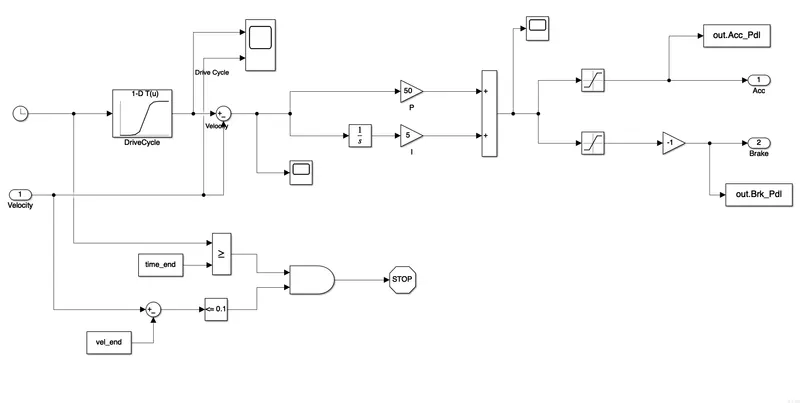
-The driver block is essentially a PI controller. It first checks the actual generated velocity from the vehicle with the velocity from the drive cycle with the help of a lookup table. The difference is then passed onto a PI controller which has a gain and integrator block and gives the change in a percentage. This output value from the PI controller can be either positive or negative depending on the current velocity of the vehicle. This value is then saturated to get the required acceleration and braking needs so that the vehicle meets the demands of the driver or in effect the drive cycle. This negative signal for the brake pedal is multiplied by -1 to make it a positive value. The sample scope output for the UDDS drive cycle is provided below. The driver block is also designed to stop the simulation if the simulation meets the end time of the drive cycle and if the velocity of the vehicle is the end velocity of the drive cycle which would basically mean we reached the end of the drive cycle.

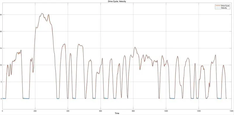
Fig 4: Scope output for comparing velocities

Controller block

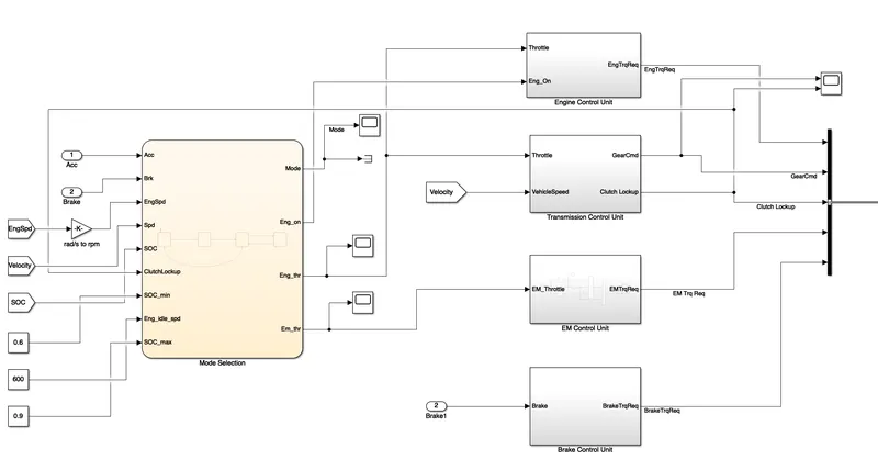
The controller block has two main parts, the mode selection block which is a logic control block to determine the state of the vehicle. In the current model, there are 4 modes which simulate the current state of the hybrid vehicle.

Working :

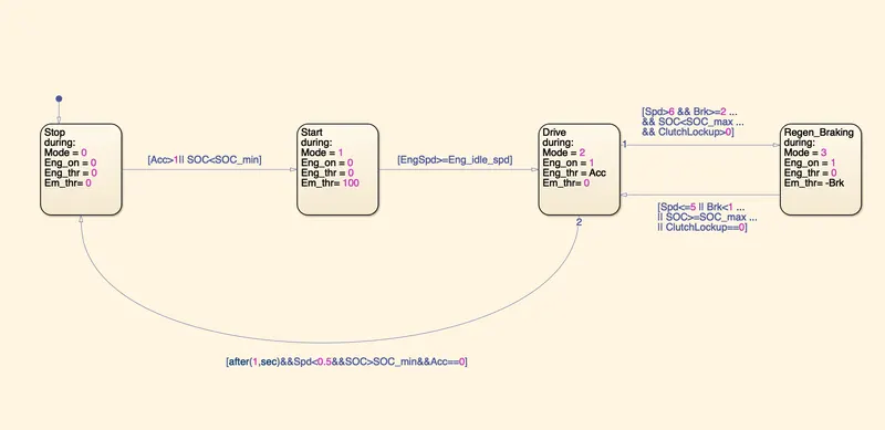
The state flow block takes in various inputs such as engine speed, acceleration and braking requirement, state of charge etc and uses them to determine the mode the vehicle is presently in. The Simulink model includes 4 modes for the vehicle which are described below

Mode 0: Stop

Mode 0 basically simulates the vehicle in the stop condition. Here the engine will be shut off, engine and motor throttle requirement is zero. It is basically used when the vehicle is at a stop signal or stopped for a brief period of time.

Mode 1: Start

Mode 1 is used to signal that the vehicle is needed to be started and moved. As a result, the Electric Motor is turned on and it will be used to start the internal combustion engine for motion. Here since the engine is still in off condition, the engine throttle is zero however motor throttle will be at a hundred percent.

Mode 2: Drive

In this mode, the engine is turned on and the vehicle starts moving. Since the engine is up and running the electric motor is turned off. The acceleration requirements for the vehicle will be solely provided by the engine.

Mode 3: Regenerative braking mode

This mode is used when the vehicle speed and brakingrequirements are above a certainthreshold provided the current SOC is less than the maximum SOC the battery can handle. On the basis of the current model, the signals such as whether the engine is on or off, engine throttle and electric motor throttle signals are givento the appropriate control units to convert them into their torque requests to be sentto the power train.

Engine Control Unit:

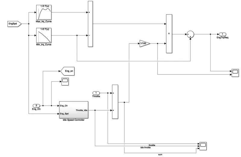
The engine control unit takes the throttle requirement as input and takes in values for engine speed and engine working condition (on or off) from ‘from tags’ and computes the engine torque request. The engine speed is passed onto two look-up tables to find out the maximum and minimum torque of the engine. This difference is then used to compute engine torque requests with the help of the throttle percentage. The idle speed controller subblock provides the throttle necessary to keep the engine idling. This value is then added with the throttle request for acceleration to provide the total torque demanded from the engine. This value is then multiplied max-min torque difference to get the engine torque demanrefer Fig 5

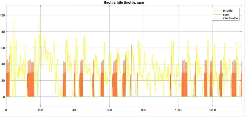
Fig 5: Scope output showing idle throttle, engine throttle for acceleration and their sum

Idle Speed Controller

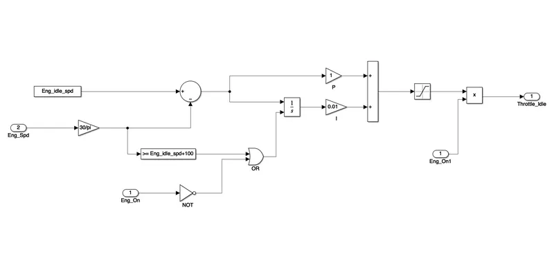
The idle speed controller block is basically a PI controller which gives the idle throttle request i.e the throttle needed to keep the engine idling so that it doesn't stall by computing the difference between the engine idle running speed and the current speed. The error is then multiplied with constant P and the integrated error is multiplied with constant I.

Transmission Control Unit

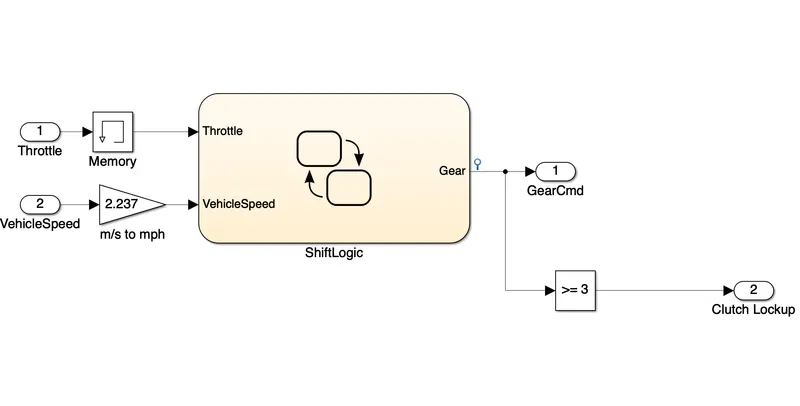
This control unit decides which gear is to be selected for the vehicle based on the throttle signal and vehicle speed. The ShiftLogic is the logic control block for defining the gear. In addition, a clutch lockup command is simulated which locks up the clutch in the torque converter unit for gears 3 and 4. Thus the pump torque will be equal to turbine torque.

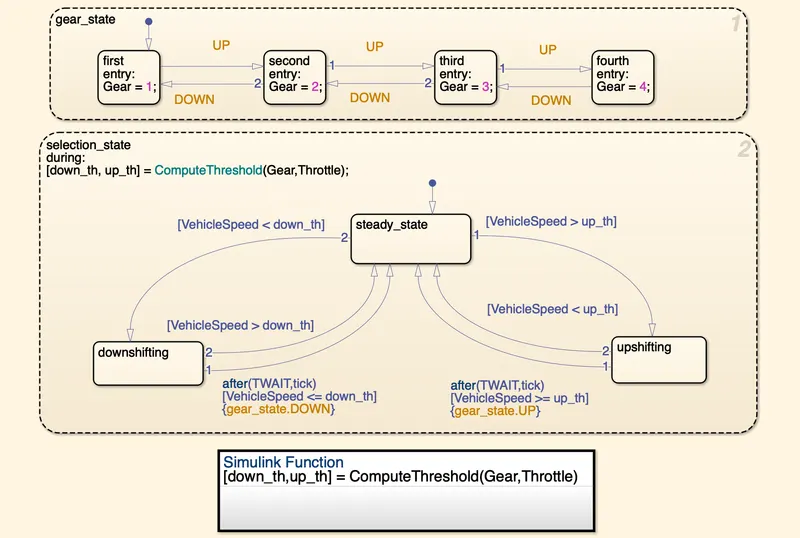
The ShiftLogic has two Stateflow diagrams. The first diagram i.e the gear_state defines 4 states as the vehicle has4 gears in total. The decision to go p ordown a gear is defined by the second state flow diagram selection_state. During the running of this block a function ComputeThreshold is run which gives thethreshold values for going up a gear or down a gear i.e up_th and down_th respectively. On the basis of this upshiftingor downshifting state is selected which gives the command to go UP or DOWN in the firstStateflow diagram.

Compute Threshold function

Shown below is threshold calculation

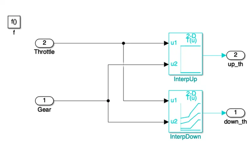
The function uses lookup tables to find the transmission shifts and provides two outputs which feed the selection_state.

EM Control Unit

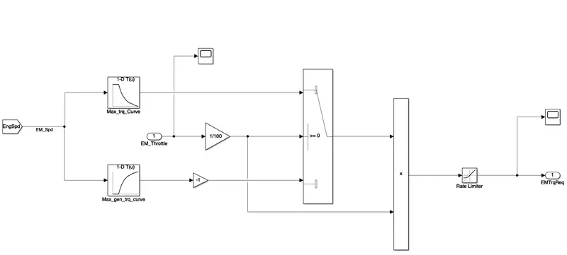
- This sunblock computes the electric motor torque required on the basis of the input EM_Throttle. First, it is checked whether the EM throttle is positive or negative. Positive values mean torque is requested from the motor and takes values from the Max torque curve with the help of a 1D look-up table else if the torque is negative, it means torque is being generated by the motor and takes values from the Max generated torque look-up table. This is made possible with the help of a switch block. A negative gain of -1 is given to the generated torque value so that the throttle request remains negative since both EM_throttle and Max generated torque values will be negative. A rate limiter is also used to control the rate at which the EM torque request increases or decreases because sudden changes in torque values are not desirable.

Brake Control Unit

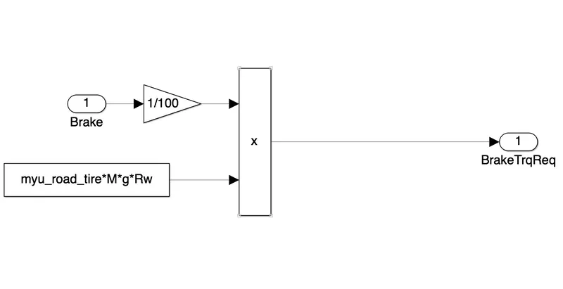
The Brake pedal signal from the Driver block is multiplied by the maximum friction, which gives the maximum braking torque. The gain block is used to convert the actual value from the percentage.

Powertrain Block

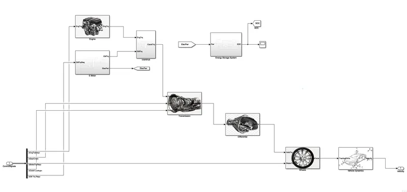
The powertrain block consists of the following subsystems: Engine, E Motor, Crankhub, Energy Storage System, Transmission, Differential, Wheels and Vehicle Dynamics. The signals from the Controller block are extracted using the bus selector, which consists of the signal for Engine torque requirement, Gear command, Brake Torque Requirement, Electric Motor Torque Requirement and Clutch Lockup.

Engine

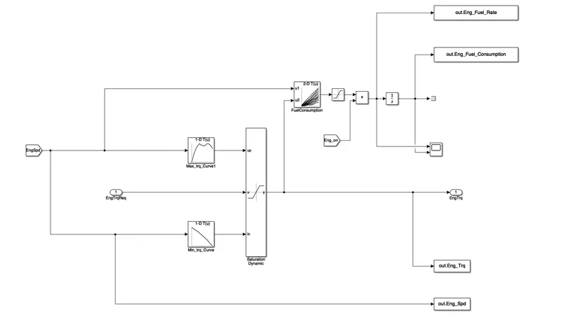
- The engine sunblock takes engine torque request as an input signal and passes it through a dynamic satration block with max engine torque curve and min engine torque curve as the limits. The maximm and minimum torque curves are found using the lookup table according to the engine speed from the data from the Matlab file "Engine_data_1_9L_Saturn_95kW". These limits are computed with the help of 1-D look-up tables which takes engine speed as input. The saturated value is the engine torque provided by the engine. The engine speed and enine outut torque are used as inputs for a 2-D lookup table to determine the instantaneous fuel rate. The saturation block ensures thatthe fuel rate vaue is positive. A subsequent integrator block is then provided to calculate the fuel consumption rate for the time engine has been running. The requiredparameters are transferred to the workpace using To Workspace blocks.

E Motor

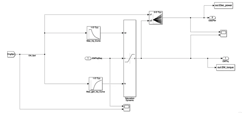
The E Motor sub-block works almost in the sameway as that of the engine block. The E Motor torquerequst from the control signal is used as input and passed through a dynamic saturation block which takes the upper and lower limits from 1 D lookup tables and gives the required Electric Motor torque as output. These limits are computed with the help of 1-D look-up tables which take engine speed or E-Motor speed (here both are the sme as in this P-1 architecture, the e motor is directly coupled to the engine without a clutch in between) as inputs. E Motor speed and E Moor generated torque is passed to a 2-D lookup table which gives the produced (in case of motoring) or generated (in case of regenerative braking) electric power. The required paramters are transferred to the workspace using To Worspace blocks.

Crank hub

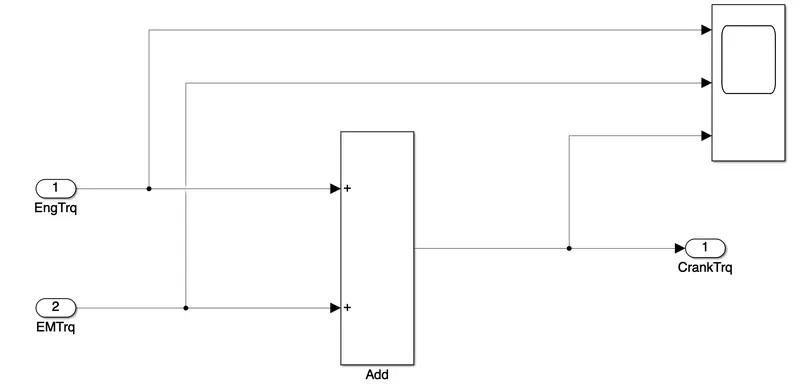
Just before supplying the generated torque to the transmission unit, there is a crank hub. This sub-block basically takes the generated Engine and E Motor torque and adds it up using a summation block. The subsequently generated torque is then passed onto the transmission block.

Transmission

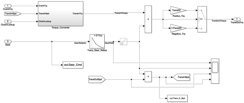
The transmission block takes Crank Torque, Clutch Lockup and Gear Command as input and computes transmission input torque with the help of a torque converter block. This Input transmission torque is then passed onto a gear system which uses the gear ratio to calculate the transmission output torque and transmission input speed. The gear ratio is selected with the help of a 1-D lookup table. The switch is used in order to consider the efficiency of the transmission. The sample output from the scope for the UDDS drive cycle is shown in the below graphfs

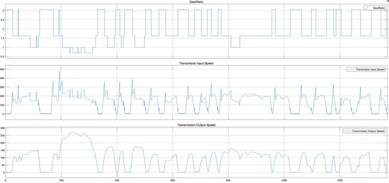
Fig 6 represents the Scope output from the Transmission subsystem.

Torque Converter

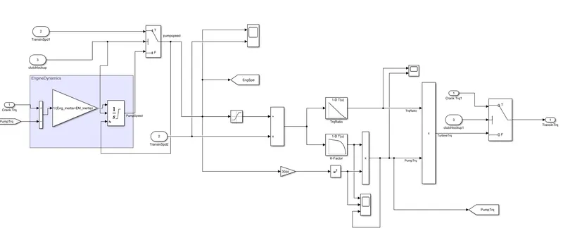
A torque converter is used because when the vehicle is stopped the engine speed can not go below a particular value as that will resultin engine stalling. So the engine must keep spinning at minimum idle speed. In addition, when torque is to be transmitted from the crank hub to the transmissionunit, it needs to be smooth otherwise a lot of vibrations will be produced. A torqueconverter also provides torque multiplication at low speeds. The fluid in the torque converter ensures a smooth transfer of torque from the engine to the transmission unit. The torque cnverter takes in crank torque, clutch lockup signal and transmission input speed as inputs. First, the pump torque is subtracted from crank hub torque as thatis the load on the engine. The subsequent value is then divided by the sum of the engine and electric motor inertia to get the acceleration. This value is then integrated to get the pump speed. A switch is used todetermine whether the pump speed is the aforementioned calculated value or the turbinespeed in case of clutch lockup is 1

The turbine speed is divided by the pump speed to get the speed ratio which is passed as input to 1-D lookup tables to get the corresponding torque ratio and capacity factor.

The capacity factor is used for finding the pump torque from the pump speed using the equation,

C factor = pump torque/pump speed

This pump torque is used to find the turbine torque using the torque ratio.

A switch is used at the end to ensure that if the clutch lockup signal is 1 then transmission input torque will be the crank hub torque since during clutch lockup crank hub torque will be directly transmitted to the turbine. In addition during clutch lockup turbine speed will be equal to pump speed. Multiple scopes are used to visualize the various parameters. The sample scope outputs are shown in Fig 7 and 8.

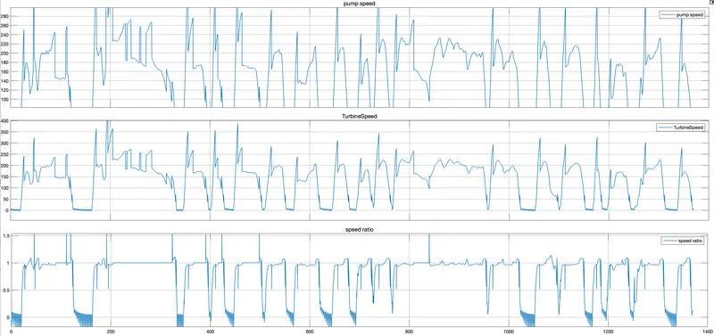
Fig 7 Scope output for analyzing pump speed, turbine speed and speed ratio of the torque converter

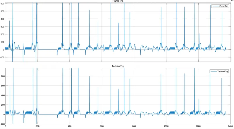
Fig 8 Scope output for analyzing Pump and Turbine Torque

Differential

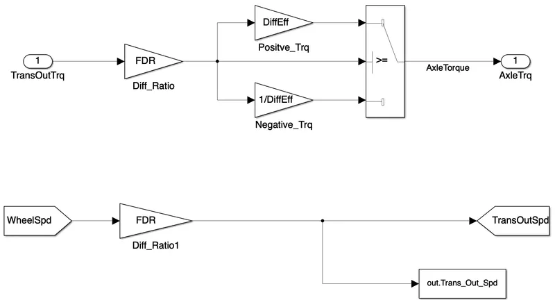
The Differential subsystem takes the output from the transmission system and reduces it as the gear ratio of the differential. The switch block is used to compensate for the negative and positive sign values. The required parameters are transferred between the other subsystems and the command window using the goto and To Workspace blocks.

Wheels

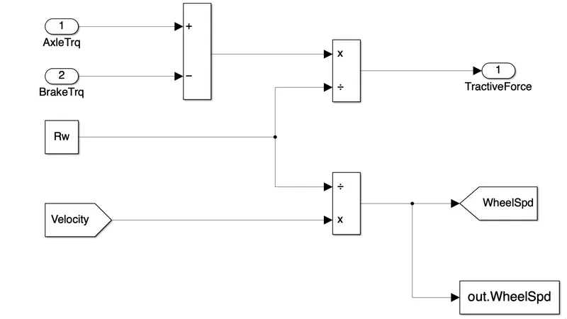
Bhe Wheels subsystem takes the axle torque and brake torque as the input. The brake torque is to reduce the axle torque to maintain the desired vehicle speed. Dividing the dynamic radius of the wheel with equivalent torque and vehicle velocity gives the tractive force and the wheel speed.

Vehicle Dynamics

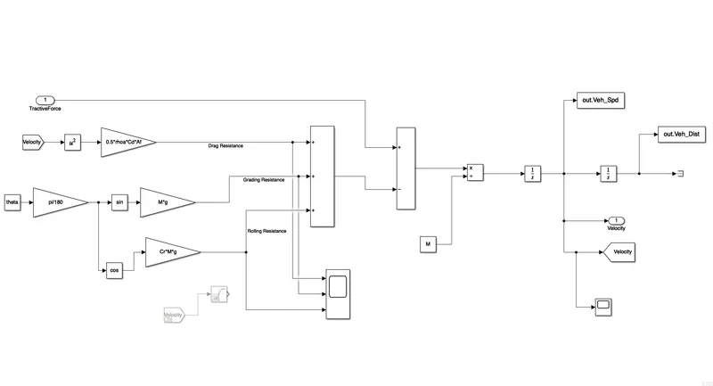
The Vehicle Dynamics block is used to determine the resultant vehicle velocity and the distance travelled. This is done by calculating the resultant force acting on the vehicle by subtracting the road load from the tractive force on the vehicle.

The road load is divided into three components i.e drag force, rolling resistance and gradient resistance.

After calculating the resultant force acting on the vehicle, the value is divided by the vehicle mass to get the vehicle acceleration which is then integrated to get the vehicle velocity which upon integration gives the distance travelled by the vehicle. The sample output from the scope for the UDDS drive cycle is shown in Figure 9. The longitudinal dynamics equation which is used for the respective block is,

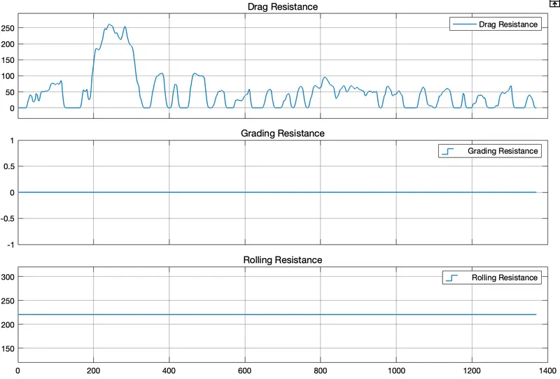
Figure 9: Scope output showing various resistance.

• Energy Storage System

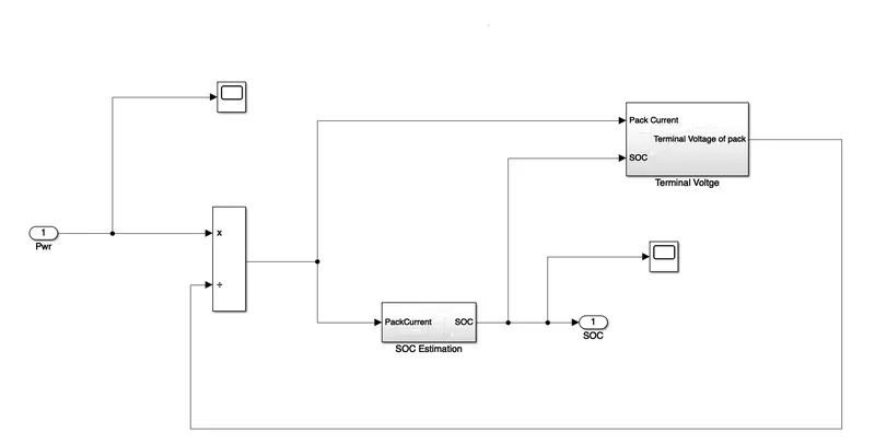
This sub-block takes electrical power generated by the E-motor as input and calculates the state of charge (SOC) of the battery pack. The SOC increases if the E-Motor is generating power and decreases if the E-Motor is producing motoring power.

The electrical power is divided by the terminal voltage to get the pack current which is then used to calculate the SOC. Terminal voltage is calculated by an equivalent circuit model.

Figure 10 shows the variation of SOC during the UDDS drive cycle.

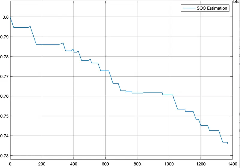
Figure 10: Variation of SOC during UDDS drive cycle

• SOC Estimation block

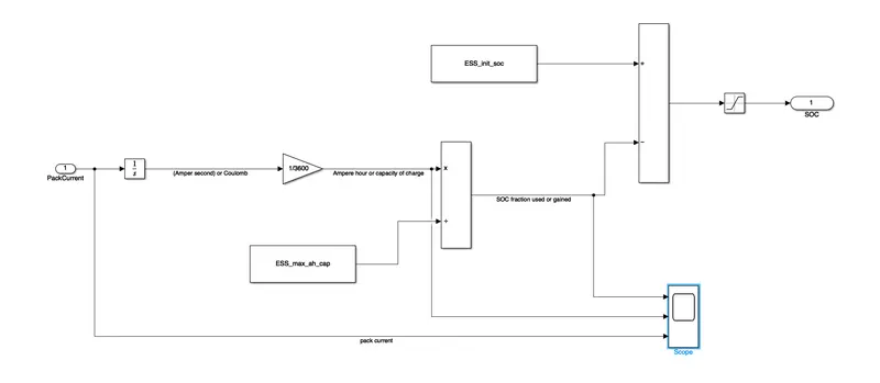
This block takes in pack current as input and calculates the SOC. Pack current is first passed through an integrator block to get the total current passed during the time period in Ampere seconds or Coulombs. A gain block is used to convert this value into Ampere hours. This capacity of charge is then divided by the maximum capacity of the battery to get the fraction of SOC used (positive) or gained (negative). This value is then added to the initial SOC value and saturated between 1 and 0 to get the current SOC value. Figure 11 shows the fraction of SOC used and gained, Capacity of charge used in ampere-hours and peak current utilised by the E-motor.

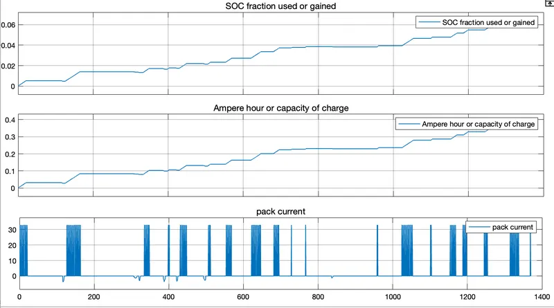
Figure 11: Scope output for SOC Estimation subblock

• Terminal Voltage Calculation

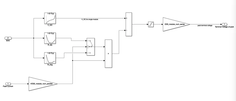
This sub-block takes in the pack current and SOC of the battery as input and calculates the Terminal voltage of the battery pack as the output using the equivalent circuit model.

The SOC value is passed through three 1-D lookup tables to calculate the corresponding open circuit voltage and module resistance during charging and discharging. A switching block is used to choose the appropriate module resistance during charging or discharging based on the sign of the module current. I.e if module current is positive. The model will take the discharge resistance value and vice versa. The pack current is divided by the number of modules in parallel to get the current passing through each module. The calculated module resistance is multiplied by the module current and the resultant value is subtracted from the open circuit voltage to get the module terminal voltage as per the following equation.

Vterminal=VOC-IR">Vterminal=VOC−IRVterminal=VOC-IR

The calculated terminal voltage of the module is then multiplied by the number of modules in series in the battery pack to get the pack terminal voltage.

Comparative Study of the Developed Model for UDDS and HWFET Drive Cycle:

Cycle kmpl (Conventional Vehicle) kmpl (P1 Hybrid Vehicle)

UDDS 11.59 12.30

HWFET 15.55 16.10

The fuel economy seemed to be significantly more for the HWFET drive cycle than the UDDS for the same vehicle characteristics. This variation is purely based on the drive cycle which is easily observable in Figures 12 and 13. The third subplot in Figures 12 and 13 gives information on the variation of velocity with respect to time. The UDDS drive cycle seems to have a more prominent varying velocity over time than HWFET. Therefore, more brake pedal has to be used for UDDS than HWFET which can be observed from the first subplot. The more the brake pedal is pressed, the more will be energy lost, which in turn means that the fuel economy number will be lesser.

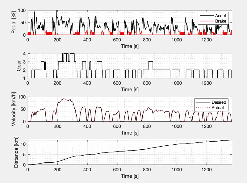
Figure 12: Vehicle Characteristics according to UDDS drive cycle

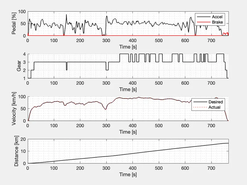
Figure 13: Vehicle Characteristics according to HWFEt drive cycle

The second subplot in Figures 12 and 13 gives information on the gear over the entire drive cycle. For the UDDS cycle, more vigorous gear shifting is observed, while for the HWFET, the gear transmission is comparatively smoother. From the fourth subplot, even though the drive cycle duration is significantly less for HWFET than UDDS, the vehicle as per the HWFET seems to have covered way more distance than the other. This is again due to the smoother velocity curve for HWFET. Also, from subplot three of Figures 12 and 13, it can be seen that the developed model was able to achieve the desired velocity, even though there are minor variations, which is obvious.

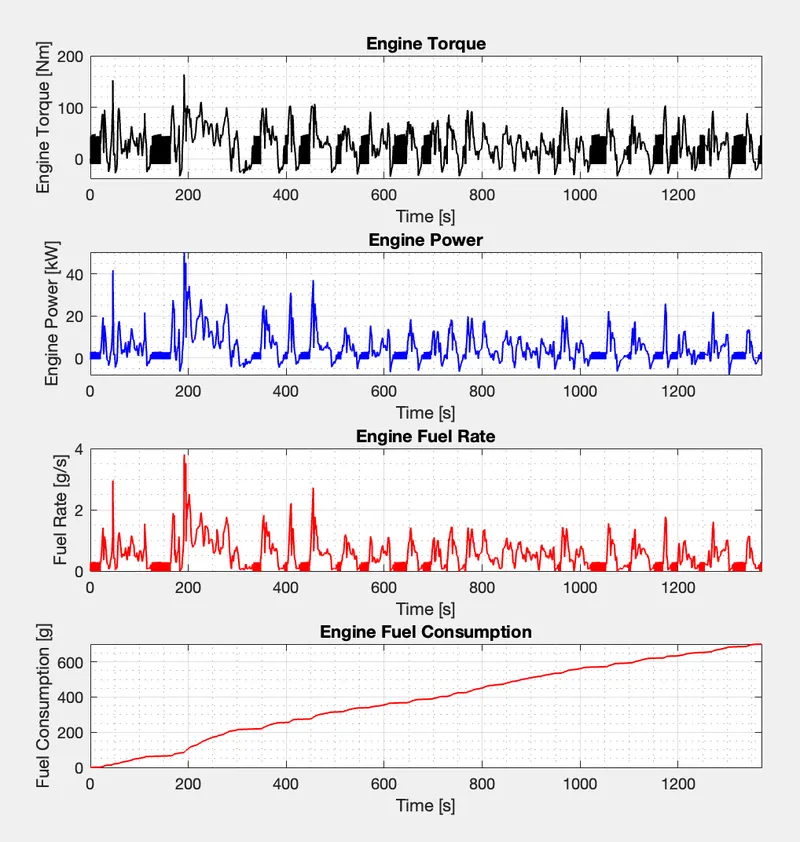
Figure 14: Engine Characteristics according to UDDS drive cycle.

The drive cycle velocity for HWFET is in the higher range than the UDDS. The power requirement is directly proportional to the power of the aerodynamic drag and directly proportional to the rolling and grading resistance. Since the proportion of higher velocity is more predominant in HWFET, the vehicle requires more power to run HWFET than UDDS, which means that, the overall fuel consumption of UDDS is less than HWFET even though the drive cycle time is more for UDDS. This can be seen in Figures 14 and 15 in subplot four. The engine torque, engine power and engine fuel rate seem to be directly proportional to each other from the Figures.

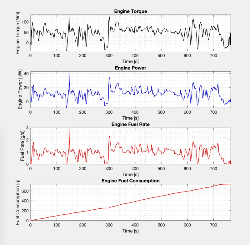
Figure 15: Engine Characteristics according to HWFET drive cycle.

Since there are frequent stops in the UDDS cycle compared to the HWFET cycle the E Motor has to work for more time in the prior case during start-stop conditions to start the engine. This is quite evident from subplots 2 and 3 from figures 16 and 17. In the HWFET cycle, there is not much power requirement from the motor as the vehicle is not stopping frequently as compared to the UDDS cycle.

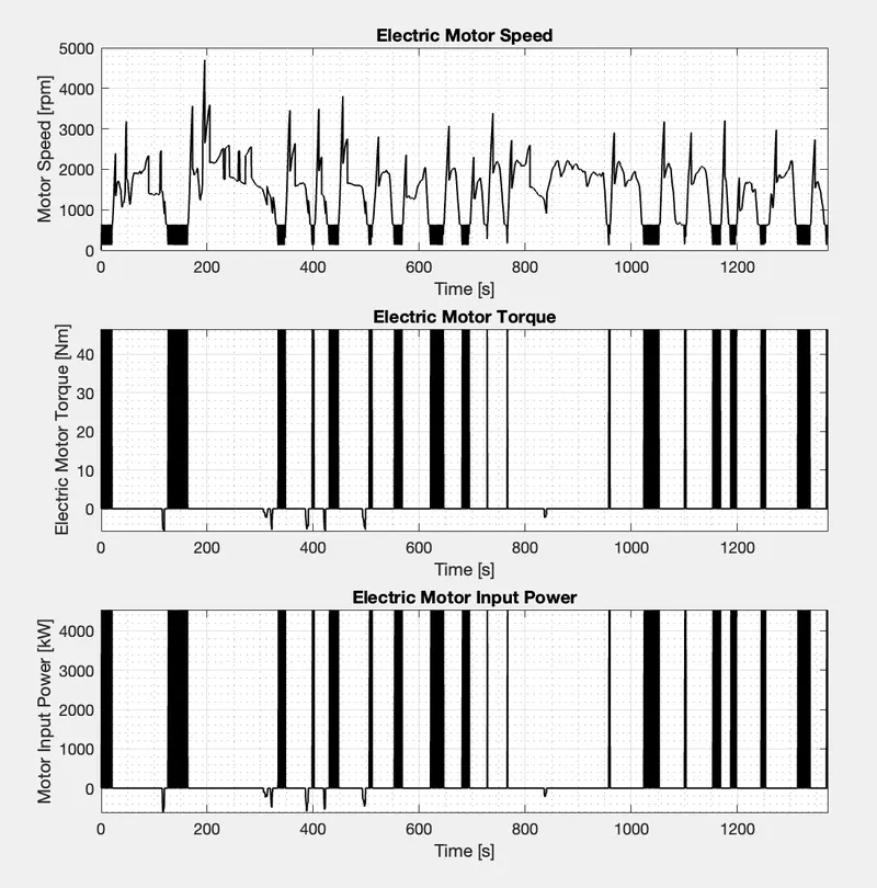
Figure 16: E-Motor Characteristics in UDDS Cycle

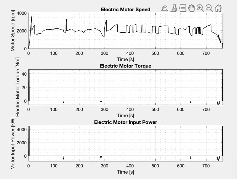
Figure 17: E-Motor Characteristics in HWFET Cycle

In the energy storage system, in the case of the UDDS cycle, the SOC of the battery pack keeps dropping as the battery pack is frequently used to start the engine and there is not much scope for the SOC to increase via regenerative breaking even though it takes place at some points. in this case, SOC generally decreases.

in the HWFET cycle, the vehicle is running mostly at a greater velocity and this provides more chance for regenerative braking which increases the SOC. this is evident from figures 18 and 19.

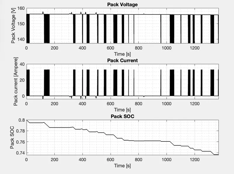
Figure 18: Battery pack Characteristics for UDDS Cycle.

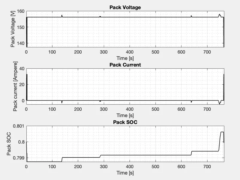
Figure 19: Battery pack Characteristics for HWFET Cycle.

The engine operating points are shown in Figures 20 and 21 for UDDS and HWFET drive cycles.

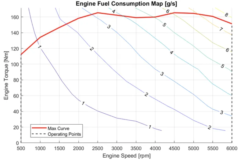
Figure 20: Engine operating points for UDDS cycle

From Figures 20, the operating points are seemed to be extreme for the UDDS drive cycle. These figures reveal that the engine is capable of going at a higher velocity than required in both drive cycles as the max engine speed possible is 6000 rpm. For the cases, the operating parameters are within the engine torque curve, and for HWFET, there are no operating points that is challenging the engine capability.

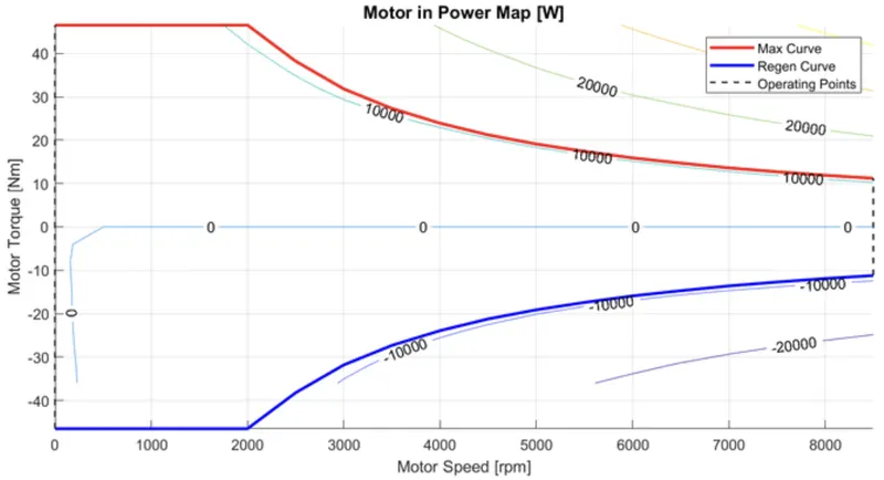
The following figures give details about the E-Motor operating characteristics. in this Simulink model, the E-Motor is going to be used for start/stop and for regenerative braking. from Motor speed of 0 to 650 rpm (engine idle speed) the motor will give 100 percent load. the points in between torques of 0 and 100 percent load is due to the rate limiter block.

The motor operating points on the motor input power map, with the motor max motoring and generating torque curves Electric motor can operates between max motoring torque curve and max generating torque curve.

Conclusion :

The Various performance of characteristics and operating point of UDDS drive cycle and HWFET drive cycle are analysed and graphs are plotted and also the MATLAB script for both initializing and post-processing has been successfully made, and a forward energy-based fuel consumption Simulink model of a Hybrid vehicle with P1 architecture is also developed successfully, and the functionality is checked. The comparative study of UDDS and HWFET for the developed vehicle model is analyzed and it was found that the P1 hybrid architectures have better fuel economy as compared to conventional vehicles.

• Time trace for engine, Transmission input, Transmission output and wheelspeed with respect to time.
• Engine torque, Engine power, Fuel rate and Fuel consumption with respect to time.
• Accelerator and brake pedal, gear command and vehicle desired, actual speed, vehicle distance with respect to time.
• Engine operating points on the engine fuel map with respect to time
• Motor speed, Torque, Motor input power with respect to time.
• Pack voltage, Current and State of charging with respect to time.
• The motor operating points on the motor input power map with respect to time.