Project 2

AIM

To analyse the performance of a P1 MHEV in MATLAB Simulink environment.

P1 MHEV (Mild Hybrid Electric Vehicle)

The powertrain configuration of the MHEV system has significant impact on the performance and characteristics of the vehicle, in terms of:

• integration cost
• fuel efficiency
• dynamic performance (powertrain torque enhancement)

Automotive OEMs and automotive Tier 1 system suppliers are currently analyzing and evaluating several major powertrain architectures for MHEVs. The electric machine can be positioned, relative to the other powertrain components, in five major points:

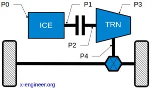
In P1 MHEV The electric machine is connected directly with the crankshaft of the internal combustion engine. Thus the engine speed and EM speed will be same.

The P1 MHEV forward model includes following systems

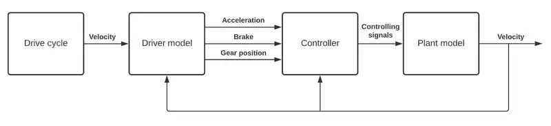
The componenets of the forward model are

• Drive cycle: It determines the driving velocity of the vehicle at a particular time, it is given in modelling window for testing and analysing the performance of the vehicle under diffrent scenario.
• Driver model: The driver model analyses the driving condition and produces the required acceleration, brake and gear position for the particular driving cycle.
• Controller: The controller takes the input command from driver model and converts it into torque request to ICE. It also gives control signal to transmission system which include gears.
• Plant model: The plant model also known as powertrain, which includes the componenets which are neccessary for the motion of the vehicle. The plant model also includes drivetrain. The controller controls the working of the plant model.

Plant model (Conventional vehicle)

Plant model consist of powertrain model of the vehicle, the componets in the plant model are mainly which are capable of producing and transferring power. The following block diagram shows the plant model of a conventional vehicle.

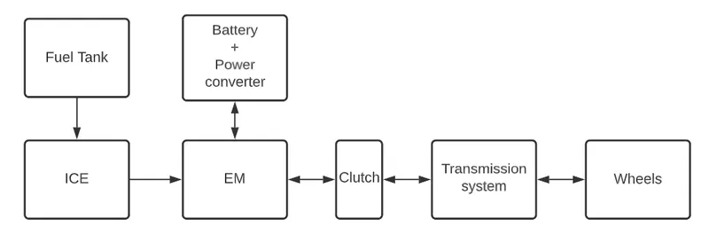
The conventional engine vehicle model is build using MATLAB Simulink as shown below.

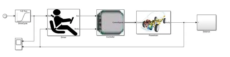
The indepth model of each subsystem are

> Driver model

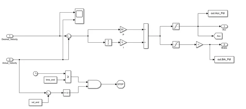
The driver model converts the input drive cycle into acceleration and brake command to the controller unit.

> Controller unit

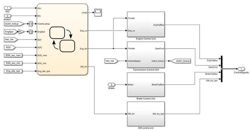
The controller unit consist of three controller

• Suprevisory controller
• Engine controller unit
• EM control unit
• Transmission controller unit (TCU)
• Brake controller unit (BCU)

>> Supervisory controller

In this controller logic an algorithm is used to supervise the other controlling unit, the unit consist of algorithm which works based on the inputs as shown in figure. The algorithm is devloped in stateflow as shown below

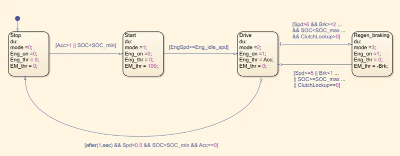
Based on the condition there are 4 mode of operation

Mode 0: idle condition

Mode 1: EM drive mode

Mode 2: Engine drive mode

Mode 3: Regenrative braking

Based on different mode the control signal are generated to each control unit to work accordingily.

>> Engine controller unit

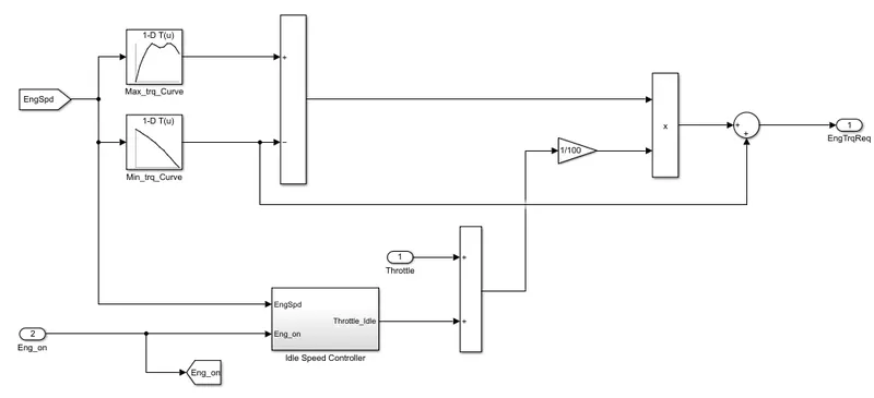
ECU generates control signal for the Engine, it gives the torque request as the signal to the engine. The torque request is proportional to the accelerartion request from the controller.

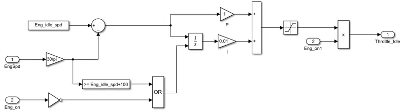
Idle speed controller

>> Transmission control unit

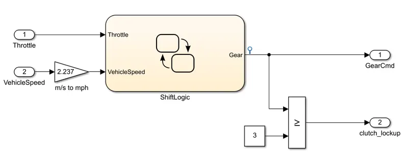
Transmission control unit consist of algorithm, by which it determines the gear position of the transmission system. The gear up shift and down shift is controlled by the TCU by using set of algorithms and conditions,

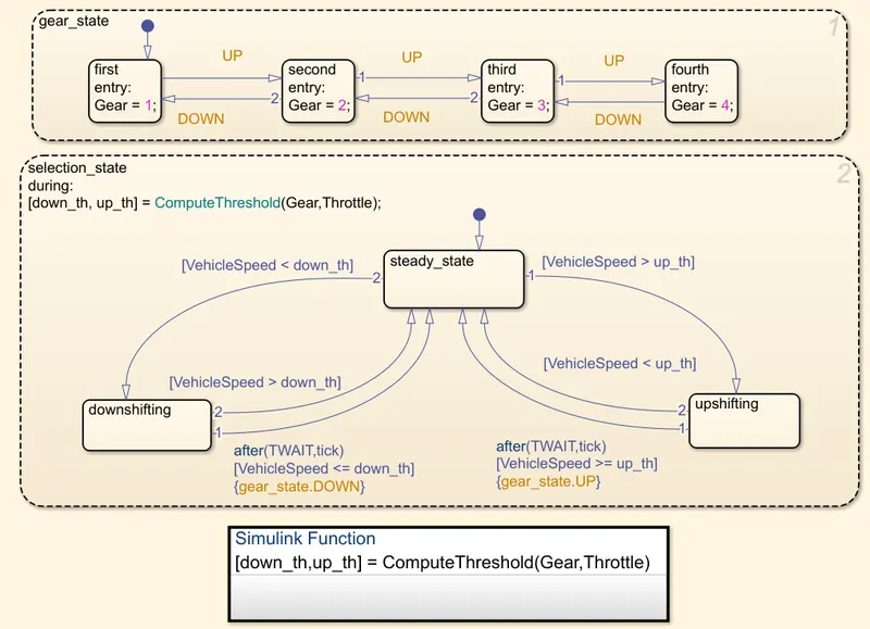
The maximum no.of gear position it have is 4, based on the velocity of vehicle and throttle response the gear shift occurs.

>> Brake control unit

The conventional engine lack off regenrative braking. The braking is done by mechanical braking using tire friction between wheels and road.

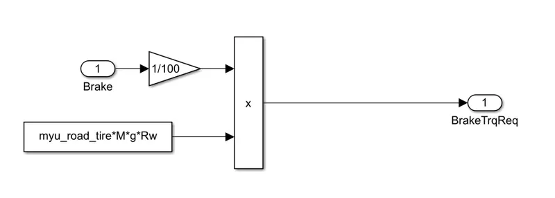
The brake request is send to the tyre, where braking is done.

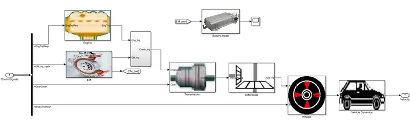
>Powertrain

The powertrain model consit of all the systems through which power is generated and flow to help the vehicle move. The powertrain model of a conventional vehicle include

• Engine
• Electric motor
• Torque coupler
• Transmission
• Differential
• Wheels
• Vehicle Power Dyanamics

>> Engine

The engine intakes fuel and convert the fuel into mechanical power required for the traction of the vehicle. The engine works based on the torque request from the ECU. It checks the torque saturation point based on the dynamic saturation limit of max torque and min torque chara obtained from a Torque-Speed chara.

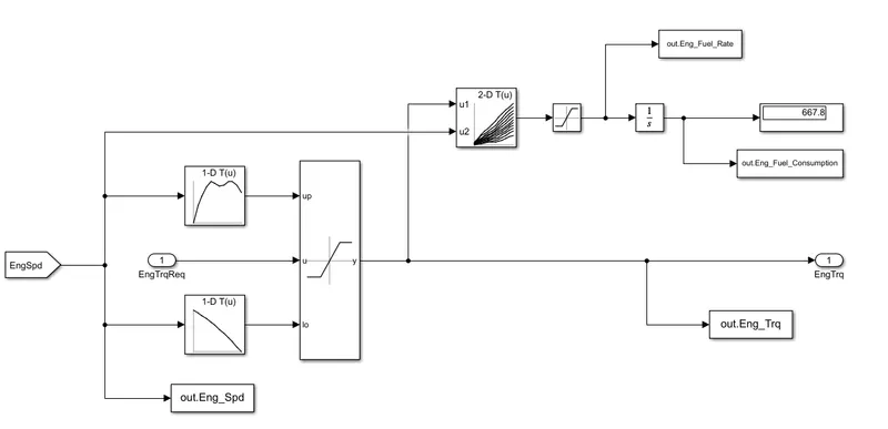
The fuel consumed is taken from 2-D chara of Speed-Torque chara, based on the speed and torque the fuel consumed is estimated, it gives fuel consumption rate in g/s, on integrating it over time it gves fuek consumed in g.

>> Electric motor

The electric motor is connected to the crankshaft of the ICE. The motor takes power from battery to support the ICE.

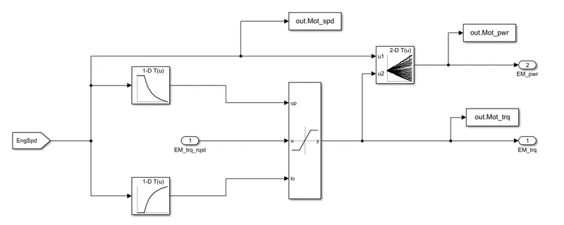
The motor performance chara is replicated with the help of 1D and 2D lookup table.

>> Battery

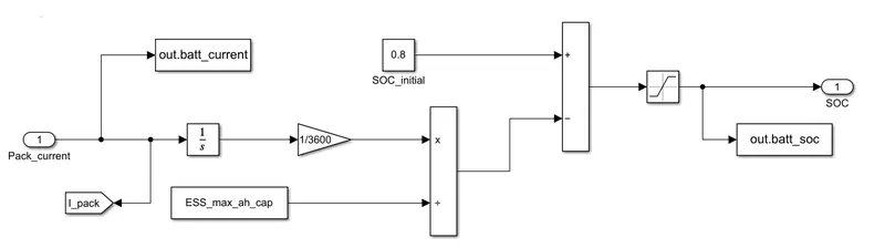
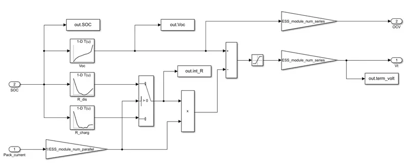
Battery act as energy storage and supplier source for the EM, when the EM powers the drivetrain the power is supplied from battery and when the EM is in regenrative mode the battery stores the energy.

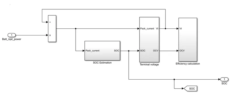
For calculating the SOC and terminal voltage following model is used

SOC estimation

Terminal voltage

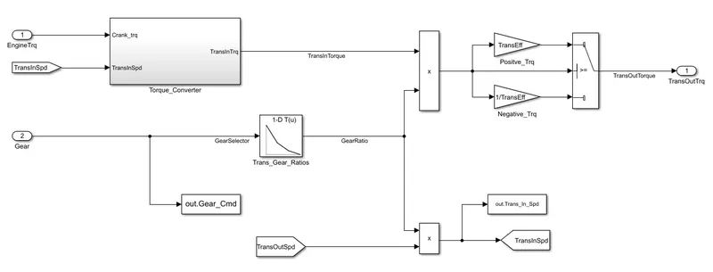
>> Transmission

The transmission is mainly used to shift gear aup and down and a clutch for isolating the engine from drivetrain during gear shift. The model of transmission is as shown below

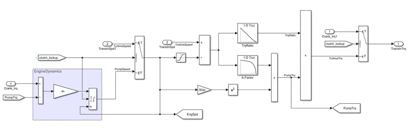
The torque converter converts the input torque from the negine into drivetrain torque.

>> Differential

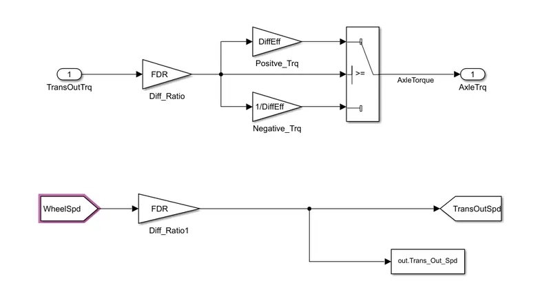
The differential transfer the power from driveshaft to the wheel axle. The differential gear ratio is given by FDR.

>>Wheels

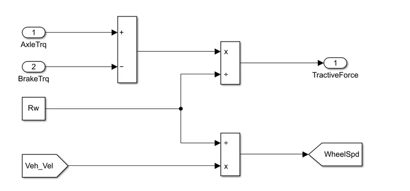
The wheel is the final place of power transfer occur between the road and vehicle. The brake torque and axle torque meets in wheels for a conventional vehicle.

>> Vehicle Dynamics

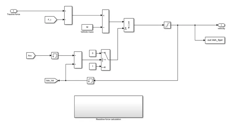
The all the forces acting on the vehicle are considered in the vehicle dynamic part. It includes the negative resistance force which effects the dynamics of the vehicle. the final output is the actual velocity of the vehicle.

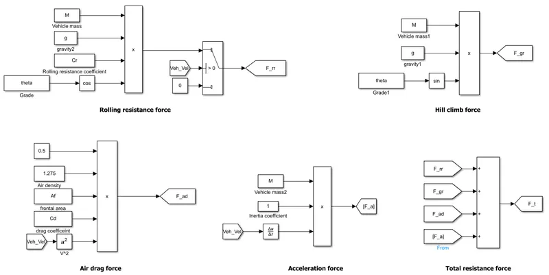
The resistive force which includes

• Rolling resistance force, Frr = Cr.M.g.Cos(a)
• Grade resistnace force, Fg = M.g.Sin(a)
• Air drag force, Fad = 0.5.Af.Cd.V^2
• Acceleration force, Fa = M.(dV/dt)

The model is given as

The total resistance force is subtracted from the tractive force, and divide by the mass of vehicle to get acceleratioj of the vehicle. On integrating the acceleration we get velocity of the vehicle.

MATLAB SIMULATION

For MATLAB simultion in Simulink, the init files are needed to load into the workspace. It can be done suing the file "Project2_InitFile.m" attached with this. in that we have different drive cycles.

%%%%%%%%%%%%%%%%%%%%%%%%%%%%%%%%%%%%%%%%%%%%%%%%%%%%%%%%%%%%%%%%%%%%%
%% Skill-Lync -> Hybrid Drives Development
% Project 1 - Conventional Vehicle Model
% By - Ullekh Gambhira 

% Description:

%% Initialization File
% Initialization file for loading the variables for the Conventional vehicle simulation model

%% Vehicle Parameters
M = 1500;       % Vehicle weight [kg]
Cr = 0.015;     % Rolling resistance coefficient
Rw = 0.35;      % Rolling radius [m]
Cd = 0.33;      % Drag coefficient
Af = 2;         % Frontal area [m2]
rhoa = 1.225;   % Air density [kg/m3]
Vwind = 0;      % Wind velocity [kmph]
g = 9.81;       % Gravitational acceleration [m/s2]
theta = 0;      % Slope [deg]
myu_road_tire = 1; % Coefficient of friction between tire - road interface

%% Powertrain Parameters 
FDR = 3.73;                         % Final Drive Ratio / Diff Ratio
DiffEff = 0.99;                     % Differential efficiency (assumed independent of operating conditions)

NumGear = 4;                        % Number of gears in transmission
TransGear = [1:NumGear];            % Transmission Gears
TransRatio = [3.06, 1.62, 1, 0.7];  % Corresponding Transmission ratios
TransEff = 0.90;                    % Transmission efficiency (assumed independent of operating conditions)

TC_SR = [0, .5, .6, .7, .8, .87, .92, .94, .96, .97, 1];   % Torque Converter Speed Ratio (Matlab default) -> TurbSpd/PumpSpd  
TC_TR = [2.232, 1.5462, 1.4058, 1.2746, 1.1528, 1.0732, 1.0192, 1, 1, 1, 1];   % Torque Converter Torque Ratio (Matlab default) -> TurbTrq/PumpTrq
TC_Cf = 1e-4 * [.72558, .66322, .63463, .59042, .51331, .4144, .29287, .22444, .12186, .04386, 0]; % Torque Converter Capacity Factor (Matlab default) -> PumpTrq/PumpSpd^2 [Nm/rpm^2]

load Vehicle_Data/Engine_data_1_9L_Saturn_95kW
load Vehicle_Data/Trans_Shift_map
load Vehicle_Data/EM_Honda_Insight_10kW
load Vehicle_Data/ESS_NiMH6


ESS_init_soc = 0.8;
ESS_soc_max = 0.9;
ESS_soc_min = 0.6;


%% Driver Parameters
Kp = 10;                    % P gain for driver PI model
Ki = 1;                     % I gain for driver PI model
Drive_Cycle_Select = 1;     % Drive cycle selection

% Drive cycle values in m/s

if Drive_Cycle_Select == 1
    load DriveCycles/UDDS;
    
elseif Drive_Cycle_Select == 2
    load DriveCycles/HWFET;
    
elseif Drive_Cycle_Select == 3
    load DriveCycles/FTP;
    
elseif Drive_Cycle_Select == 4
    load DriveCycles/US06;
    
elseif Drive_Cycle_Select == 5
    load DriveCycles/NEDC;
    
elseif Drive_Cycle_Select == 6
    load DriveCycles/WLTP;
 
end

time_end = cyc_time(end);
vel_end = cyc_vel(end);

Drive cycle code:

1 - UDDS

2 - HWFET

3 - FET

4 - US06

5 - NEDC

6 - WLTP

After selecting loading the init file with required drive cycle, simulate the model in simulink window.

After simulation for analysing the result use the anlaysing mscript file "Project2_ProcessingFile.m", attached with this

%%%%%%%%%%%%%%%%%%%%%%%%%%%%%%%%%%%%%%%%%%%%%%%%%%%%%%%%%%%%%%%%%%%%%
%% Skill-Lync -> Hybrid Drives Development
% Project 1 - Conventional Vehicle Model
% By - Ullekh Gambhira 

% Description:
% The following file is to used with the Initialization file and Simulink
% results for post-processing of the data.
% The file is incomplete, has some examples of how the data is imported
% into a readable format, data analysis and plotting examples.
% Based on the project task, use commands in a similar format as given
% below, to analyse the data and generate required plots.
% You can change variable names if desired

%% Post-Processing File
%  File for post-processing the Conventional vehicle simulation model data

%% Renaming variables
Time = out.tout;
Acc_Pdl = out.Acc_Pdl;          % Accelerator pedal [%]
Brk_Pdl = out.Brk_Pdl;          % Brake pedal [%]
Gear_Cmd = out.Gear_Cmd;        % Transmission gear
Trans_In_Spd = out.Trans_In_Spd*30/pi;  % Transmission input speed [rpm]
Trans_Out_Spd = out.Trans_Out_Spd*30/pi;% Transmission output speed [rpm]
Eng_Trq = out.Eng_Trq;          % Engine brake torque [Nm]
Eng_Spd = out.Eng_Spd*30/pi;    % Engine speed [rpm]
Eng_Fuel_Consump = out.Eng_Fuel_Consumption;    % Engine fuel consumption [g]
Eng_Fuel_Rate = out.Eng_Fuel_Rate;      % Engine fuel rate [g/s] 
Veh_Dist = out.Veh_Dist/1000;   % Distance traveled by vehicle [km]
Veh_Spd = out.Veh_Spd*18/5;     % Vehicle speed [kmph]
Des_Spd = cyc_vel*18/5;         % Desired vehicle speed [kmph]
Wheel_Spd = Trans_Out_Spd/FDR;  % Wheel speed in [rpm]
Mot_spd = out.Mot_spd;          % motor speed [rpm]
Mot_trq = out.Mot_trq;          % motor torque [Nm]
Mot_pwr = out.Mot_pwr/1000;     % motor power [kW]
Batt_amp = out.batt_current;    % battery pack current [A]
Batt_vt = out.term_volt;        % battery terminal voltage [V]
Batt_soc = out.batt_soc*100;    % battery soc level

%% Data Analysis
Eng_Pwr = (Eng_Spd*pi/30).*Eng_Trq/1000;   % Engine brake power [kW]
rho_petrol = 0.7197;                    % Density of petrol [kg/L]
kmpl = Veh_Dist(end)/(Eng_Fuel_Consump(end)/1000/rho_petrol);    % Fuel economy [kmpl] 


%% Time trace for engine, transmission input, transmission output and wheel speed on one plot.
figure();
plot(Time,Eng_Spd,'linewidth', 1);
hold on
plot(Time,Trans_In_Spd,'linewidth', 1);
hold on
plot(Time,Trans_Out_Spd,'linewidth', 1);
hold on
plot(Time,Wheel_Spd,'linewidth', 1);
hold on
legend('Engine Speed','Transmission input speed','Transmission output speed','Wheel sppeed');
xlabel('Time [s]');
ylabel("Speed [rpm]");
title("Engine, transmission input, transmission output and wheel speed");

%% Plotting engine torque, engine power, fuel rate and fuel consumption
figure()
subplot(4,1,1)
hold on
grid on
plot(Time, Eng_Trq, 'linewidth', 1, 'Color', 'red');
title("Engine Torque");
ylabel('Torque [Nm]')
xlim([0, Time(end)]);
subplot(4,1,2)
hold on
grid on
plot(Time, Eng_Pwr, 'linewidth', 1, 'Color', 'blue');
title("Engine Power");
ylabel('Power [W]')
xlim([0, Time(end)]);
subplot(4,1,3)
hold on
grid on
plot(Time, Eng_Fuel_Rate, 'linewidth', 1, 'Color', 'magenta');
title("Engine Fuel consumption rate");
ylabel('Fuel rate [g/s]')
xlim([0, Time(end)]);
subplot(4,1,4)
hold on
grid on
plot(Time, Eng_Fuel_Consump, 'linewidth', 1, 'Color', '#006400');
title("Engine Fuel Consumption");
xlabel('Time [s]');
ylabel('Fuel [g]');
ylim([0,800]);
xlim([0, Time(end)]);


%% Plotting vehicle characteristics time accelerator and brake pedal, gear command, vehicle desired and actual speed, vehicle distance
figure('Name','Vehicle Characteristics')
hold on
grid on
subplot(2,2,1)
hold on
grid on
plot(Time, Acc_Pdl, 'linewidth', 1, 'Color', 'black');
plot(Time, Brk_Pdl, 'linewidth', 1, 'Color', 'red');
ylabel('Pedal [%]')
xlim([0, Time(end)]);
legend('Accel','Brake');
title("Acceleration and Brake command");
subplot(2,2,2)
hold on
grid on
plot(Time, Gear_Cmd, 'linewidth', 1, 'Color', 'black');
xlim([0, Time(end)]);
xlabel('Time [s]');
ylabel('Gear');
title("Gear position");
subplot(2,2,3)
hold on
plot(cyc_time,Des_Spd,'LineWidth',1,'Color','blue');
plot(Time,Veh_Spd,'LineWidth',1,'Color','red');
legend("Desired velocity","Actual velocity");
ylabel("Velocity [kmph]");
xlabel("Time [s]");
title("Desired vs Actual velocity");
subplot(2,2,4);
hold on
plot(Time,Veh_Dist,'LineWidth',1,'Color','black');
ylabel("Distance [km]");
xlabel("Time [s]");
title("Distance travelled")


%% Plotting engine operating points on engine fuel map
figure('Name','Engine Operating Points');
hold on
grid on
title('Engine Operating Points','fontsize',12);
p1=plot(Eng_map_spd*30/pi,Eng_max_trq,'linewidth',2,'color','r');
p2=line([Eng_map_spd(end)*30/pi Eng_map_spd(end)*30/pi],[0 Eng_max_trq(end)]);
set(p2,'linewidth',1,'linestyle','--','color','k');
p3=line([Eng_map_spd(1)*30/pi Eng_map_spd(1)*30/pi],[0 Eng_max_trq(1)]);
set(p3,'linewidth',1,'linestyle','--','color','k');
[c,h] = contour(Eng_map_spd'*30/pi,Eng_map_trq,Eng_fuel_map');
clabel(c,h);
xlabel('Engine Speed [rpm]');
ylabel('Engine Torque [Nm]');
title('Engine Operating Points');
p4 = plot(Eng_Spd,Eng_Trq,'.','color','k');
legend([p1 p4],{'Max Curve','Operating Points'});
axis([Eng_map_spd(1)*30/pi Eng_map_spd(end)*30/pi 0 Eng_map_trq(end)]);


%% Plotting motor speed, torque, motor input power using subplots
figure("Name","Speed at different stages")
subplot(3,1,1)
plot(Time,Mot_spd,'linewidth', 1);
ylabel("Speed [rpm]");
title("Electric motor Speed");
subplot(3,1,2)
plot(Time,Mot_trq,'linewidth', 1);
ylabel("Torque [Nm]");
title("Electric motor torque");
subplot(3,1,3)
plot(Time,Mot_pwr,'linewidth', 1);
ylabel("Power [kW]");
title("Electric motor input power");
xlabel('Time [s]');


%% Battery parameter
figure("Name","Battery parameters")
subplot(3,1,1)
plot(Time,Batt_vt,'linewidth', 1);
ylabel("Voltage [V]");
title("Battery terminal voltage");
subplot(3,1,2)
plot(Time,Batt_amp,'linewidth', 1);
ylabel("Current [A]");
title("Battery pack current");
subplot(3,1,3)
plot(Time,Batt_soc,'linewidth', 1);
ylabel("SOC [%]");
title("Battery SOC level");
xlabel('Time [s]');


%% Plotting Electric motor operating points
figure('Name','Motor Operating Points');
hold on
grid on
title('Engine Operating Points','fontsize',12);
q1=plot(EM_map_spd*30/pi,EM_max_trq,'linewidth',1,'color','red');
q4=plot(EM_map_spd*30/pi,EM_max_gen_trq,'linewidth',1,'color','blue');
q2=line([EM_map_spd(end)*30/pi EM_map_spd(end)*30/pi],[0 EM_max_trq(end)]);
set(q2,'linewidth',1,'linestyle','--','color','k');
q3=line([EM_map_spd(1)*30/pi EM_map_spd(1)*30/pi],[0 EM_max_trq(1)]);
set(q3,'linewidth',1,'linestyle','--','color','k');
[c,h] = contour(EM_map_spd'*30/pi,EM_map_trq,EM_inpwr_map');
clabel(c,h);
xlabel('EM Speed [rpm]');
ylabel('EM Torque [Nm]');
title('EM Input Power');
p5 = plot(Mot_spd,Mot_trq,'.','color','k');
legend([q1 q4 q3],{'Max Curve','Regen Curve','Operating Points'});

After running the above MATLAB script file required results can be obtained.

Lets consider two cases with drive cycle as UDDS and HWFET.

CASE 1: UDDS drive cycle

For loading UDDS drive cycle, edit the "Drive_Cycle_Select = 1;" in the init file. Now run the init model, and simulate the model.

For analysing the result run the "Project1_processing.m" file, the following results are obtained.

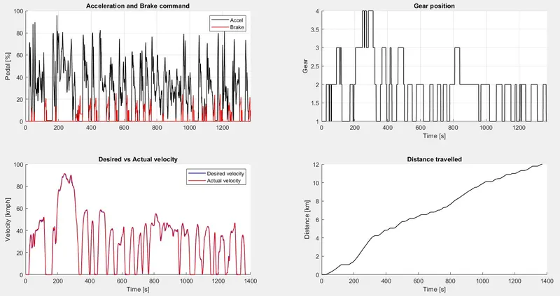
a. Accelerator and brake pedal, gear command, vehicle desired and actual speed, vehicle distance

Observation

• In UDDS cycle the acceleration and brake commands are frequent.
• The gear position mostly is in 2nd and 1st due to frequent stop and go drive pattern.
• The desired and actual velocity match each other, it shows the good dynamic behaviour of the powertrain of the vehicle.

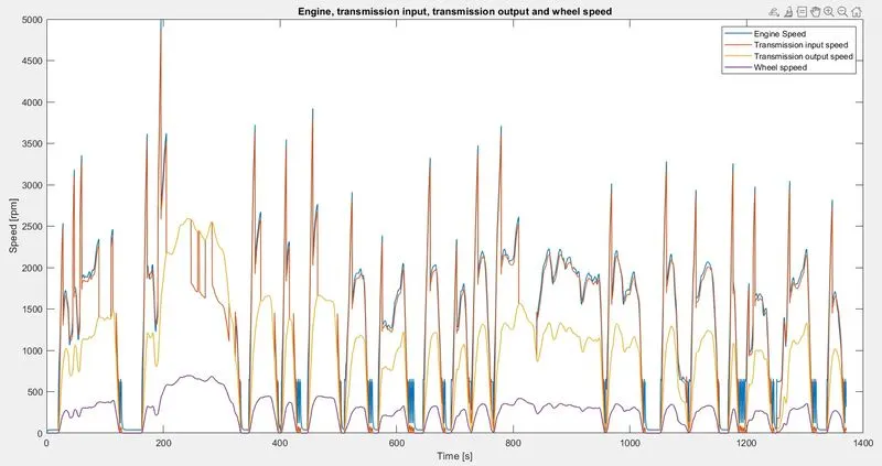
b. Time trace for engine, transmission input, transmission output and wheel speed

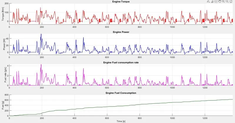
c. Engine torque, engine power, fuel rate and fuel consumption using subplots.

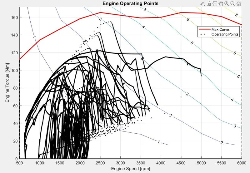
d. Engine operating points on the engine fuel map.

>> P1 MHEV engine operating point

>> Conventional vehicle engine operating point

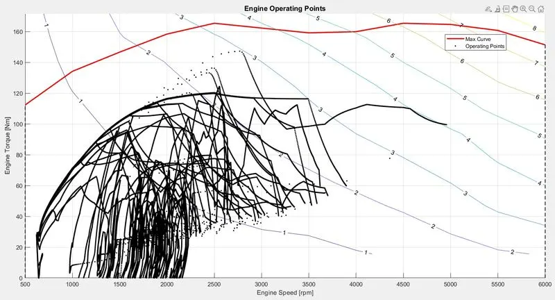
Observation:

• The engine operating points at different times are shown in black mark.
• The operating points are wide in range, due to lots of starts and stops in the drive cycle.
• There is not much difference in the operating point of a P1 MHEV and a normal conventional vehicle engine operating points as in this model the role of EM is very less.

e. Plot motor speed, torque, motor input power using subplots.

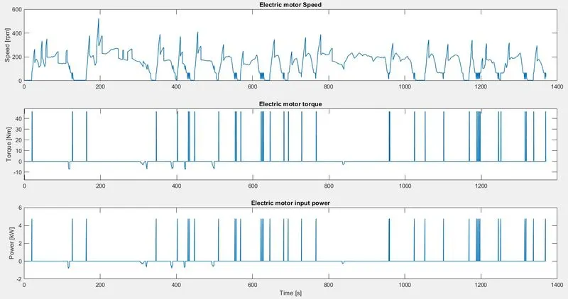
Observation

• The EM is less frequently used whenever the vehicle starts from rest and during the regenerative braking.

f. Plot pack voltage, current and SoC using subplots.

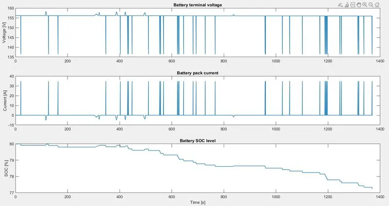
Observation:

• The SOC of battery decreases as the power supported by the EM during starting is greater, and the regenrative braking is less.

g. Plot the motor operating points on the motor input power map, with the motor max motoring and generating torque curves.

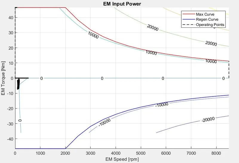
Observation:

• The EM operating point is at max at starting of vehicle near to 40Nm at lower speed, thus taking advantage of high torque at starting from the EM which ICE can't support.
• In regenerative braking the negative torque is between 0 to 10Nm, which converts into electrical energy stored in battery.

Case 2: HWFET drice cycle

For loading HWFET drive cycle, edit the "Drive_Cycle_Select = 2;" in the init file. Now run the init model, and simulate the model.

For analysing the result run the "Project2_processing.m" file, the following results are obtained.

a. Accelerator and brake pedal, gear command, vehicle desired and actual speed, vehicle distance

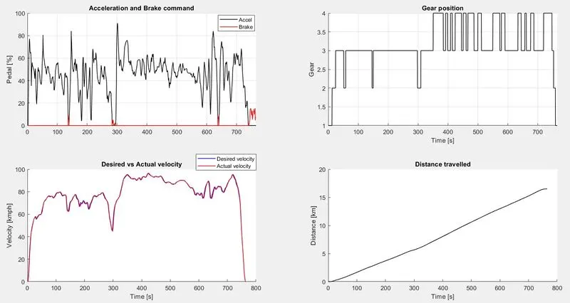
Observation

• In HWFET cycle the acceleration and brake commands are less and keep a good average high speed.
• The gear position mostly is in 3rd and 4th due to high speed drive pattern.
• The desired and actual velocity match each other, it shows the good dynamic behaviour of the powertrain of the vehicle.

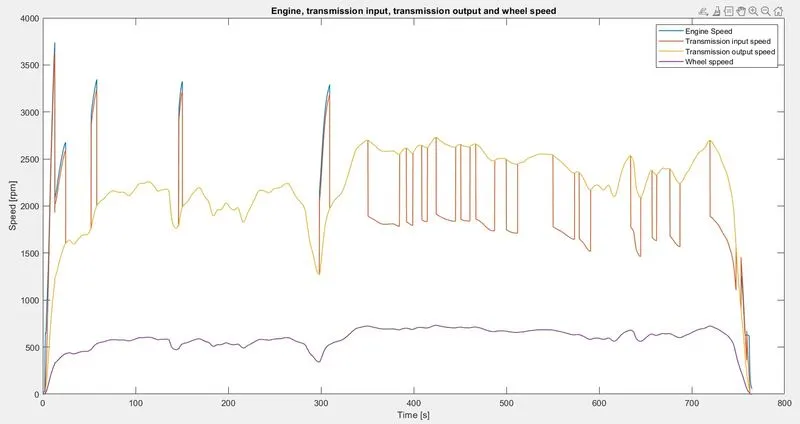
b. Time trace for engine, transmission input, transmission output and wheel speed

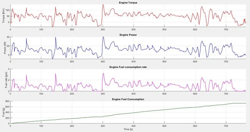
c. Engine torque, engine power, fuel rate and fuel consumption using subplots.

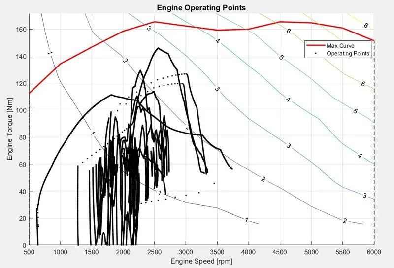
d. Engine operating points on the engine fuel map.

>> P1 MHEV engine operating point

>> Conventional vehicle engine operating point

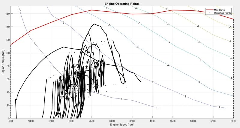
Observation:

• The black marks indicates the engine operating points at different time.
• The operating points range is narrow due to loess stop and go.
• There is not much difference in the operating point of a P1 MHEV and a normal conventional vehicle engine operating points as in this model the role of EM is very less.

e. Plot motor speed, torque, motor input power using subplots.

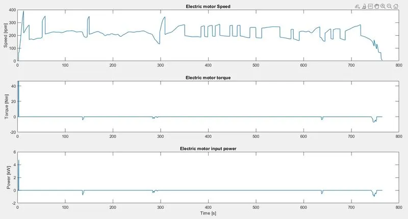
Observation:

• In this at starting the EM supports powertrain and afterwards it supports only regenrative braking.

f. Plot pack voltage, current and SoC using subplots.

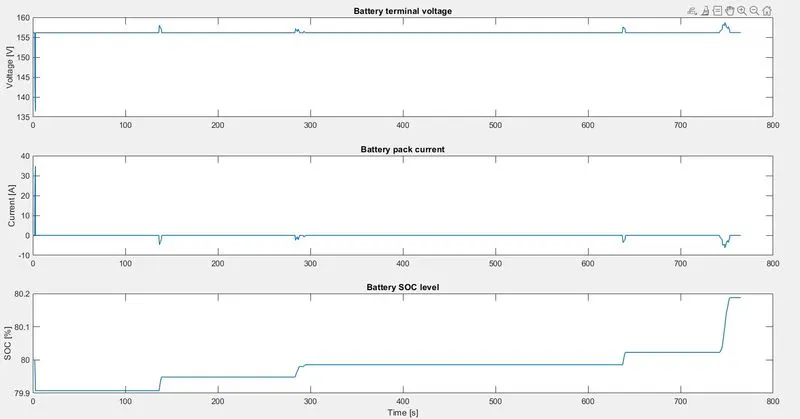
Observation:

• At starting the EM supports the powertrain and later it supports regenerative braking and hence at starting the SOC decreases and then SOC increases due to regenrative braking.

g. Plot the motor operating points on the motor input power map, with the motor max motoring and generating torque curves.

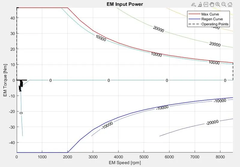
Observation:

• The EM operating point is at max at starting of vehicle near to 40Nm at lower speed, thus taking advantage of high torque at starting from the EM which ICE can't support.
• In regenerative braking the negative torque is between 0 to 10Nm, which converts into electrical energy stored in battery.

OBSERVATION AND COMPARISON:

• Drive cycle

  • Cycle	Duration	Max speed	Average speed	Distance
    UDDS	1372s	91.25kmph	31.5kmph	12.07km
    HWFET	765s	96.5kmph	77.7kmph	16.45km

• Acceleration, Brake and Gear command
  • In UDDS drive cycle, the vehicle on a average runs most in 2nd gear while in HWFET its in 3rd and 4th gear.
  • There is lots of acceleration and brake in UDDS cycle, while HWFET cycle have very less brake commands.
• Engine, Transmission input and Transmission output and Wheel speed.
  • The engine and transmission input speed [rpm] have good dynamic response, it will accelerate and deccelerate quickyl as shown in the figure.
  • The transmission output and wheel speed [rpm] dynamic response is low, because the inertia of the vehicle body as body of vehicle directly interacts with the wheel and transmission output. The transmission system seperates the engine and transmission output and thus the body interaction is not directly occurs to the engine speed.
  • The wheel speed is less compare to the transmission output because of differential gear ratio.
  • The variation of angular velocity of the system in UDDS cycle is gigh and in HWFET is low.
  • The angular velocity fluctuates between 0 and high intermittently, and thus avaerage angualr speed is less in UDDS even both have nearly same highest engine speed.
• Engine torque, power, fuel rate and fuel consumption.
  • The maximum engine torque and power is required in UDDS cycle than HWFET cycle.
  • The fuel rate is maximum for UDDS cycle nearly 4.2g/s, while HWFET max fuel rate required is 3g/s.
  • The fuel consumption is more for UDDS cycle than HWFET cycle.

  • Cycle	kmpl (conventional vehicle)	kmpl (P1 MHEV)
    UDDS	12.924	13.87
    HWFET	15.805	16.41

  • In terms of mileage HWFET gives more mileage than UDDS, because UDDS cycle is urban type HWFET is highway.
  • The mileage of P1 MHEV is more than the normal conventional vehicle with same parameter and conditions, thus hybrid EVs are more efficient compared to conventional ICE vehicle.
• Operating points of ICE
  • With same engine in different drive cycle, the operating point of engine has wide range in UDDS cycle than HWFET which have narrow range.
  • Thus the engine operates at good efficiency during constant speed or speed within a range.
• EM torque, power and speed
  • The EM speed is same as that of the ICE as both are having same shaft due to P1 configuration,
  • The EM supports at starting of the vehicle where high torque is required, and thus it have good dynamic performance than the ICE only vehicle.
  • The regenrative braking helps in converting the brake energy into electrical energy which stores in battery.
• EM operating point
  • The EM operating point is at lower rpm, as the EM supports the vehicle at starting and regenerative braking.
• Battery
  • The battery helps in powering the EM, and it also stores enegy during regenerative braking.

CONCLUSION:

A conventional vehicle has been modelled using MATLAB Simulink, the model is used to analyse the engine, powertrain and vehicle performance. The following conclusion can be made

• The engine operating point is wide for UDDS cycle compared to the HWFET cycle.
• The fuel economy of vehicle in UDDS cycle is 13.87kmpl while for HWFET is 16.41kmpl. The HWFET has good fuel economy than UDDS cycle.
• The fuel economy is greater than the ICE vehicle.
• The engine and EM average rpm of the vehicle is good for HWFET cycle compared to UDDS cycle.
• The speed variation between desired and actual for both cycles are very less compared to normal conventional vehicle at high acceleration also because of good dynamic performance of P1 MHEV.
• The vehicle is able to produce enough torque and power to meet both the drive cycles.
• The brake command is shared by the regenerative braking and the mechanical braking.
• The regenerative braking helps in conserving the brake energy into chemical energy stored in battery through EM.