Project 2
Description:
As discussed in Lecture 11, Project 2 deals with the development of a forward energy-based fuel consumption model of a P1 hybrid vehicle. This model is based on the conventional vehicle model from Project 1.
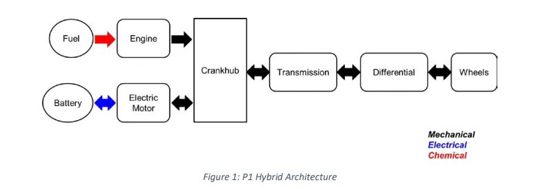
The main goal of this project is to understand the functionality of a P1 hybrid and be able to model it.
Honda Insight motor and battery are considered for this project. Data is taken from ADVISOR data base developed by NREL, USA. Data provided in the project files.

“Project2_InitFile.m” is a Matlab script used to load all the variables required for running the Simulink model and for post-processing. The drive cycle selection is also done here. Before running the Simulink vehicle model, run this initialization script.
- Layout Of Hybrid vehicle
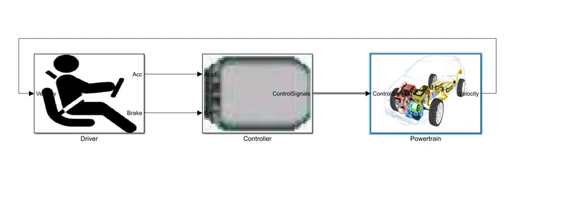
fig- Basic Layout of HEV
- Driver
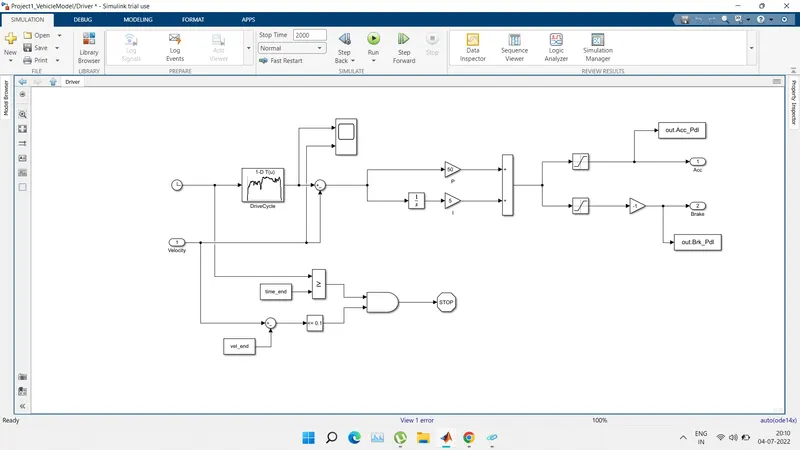
fig-Driver
It is modeled using a Driver block, which is a basic PI controller that generates accelerator and brake pedal outputs to match the desired and actual vehicle speeds. In this we use drive cycles fro the based on these results of fuel consumption and emissions the vehicle gets certified and it also forms a basis of uniform asessment. It is based on time, velocity then its all integrate and creates output accelration pedal and brake pedal.
- Controller:
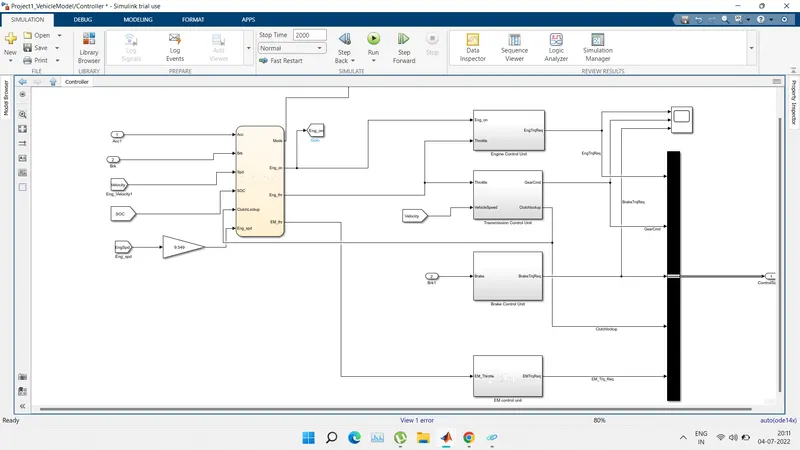
fig-controller
The Controller block is the brains of the vehicle, representing the electronic controls units. It is based on the driver inputs, it generates desired engine torque, desired transmission gear desired motor torque and desired brake torque. These inputs are fed to the 'Powertrain' block which represents the drivetrain of the vehicle. In this we require to create stateflow block it explain in next figure.
- State flow chart
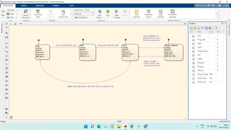
fig- State flow chart
In this we created four conditions as stop, start, drive and regenration braking. The initial block represent the stop condition. In which the engine is off. The engine and motor throttle conditions are zero. Then the second block represent start condition, in which the mode is 1 the electric motor throttle is only used to provide the required torque and power to the vehicle. the engine is off and engine throttle conditionis zero. The state 1 and state 2 are connected using the links ie, it moves from state 1 to state 2 when acceleration is less than one or SOC is less then the minimum SOC. State 3 Represtents mode 2 ile, engine is on and the engine throttle is also having positive value from the driver but the electric motor throttle is zero. It changes form state 2 to state 3 when engine speed is graeter than or equal to engine idle speed. state 4 represents regenrative braking which is model 3 in this state the engine is on but the engine throttle is having no input from driver whereas the electric moto receives the negative power due to braking. The inputs are given to chart is Acceleration, barke, engine speed, vehicle speed, SOC, and clutch lockup. The output we get from the chart is mode, engine condition, engine throttle condition, and electric motor throttle condition. Modification done in all Unit modeling, they showed in next figures.
- Engine control unit
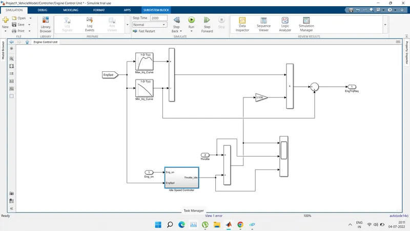
fig-engine control unit
- Transmission control unit
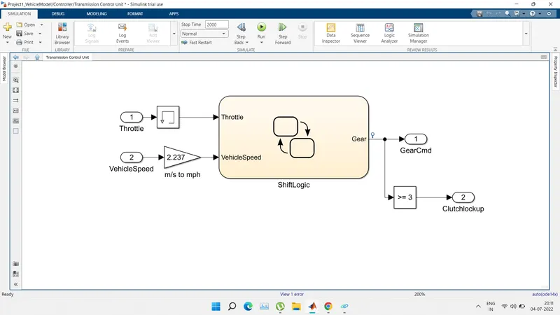
fig- Transmission control unit
In this unit we create steadly flow variable state for controlling of gears of vehicle as in ascending and descending order with respect to time, speed, distance, and give input to this steady state is vehicle speed in m/s to mph.
- Shift logic unit
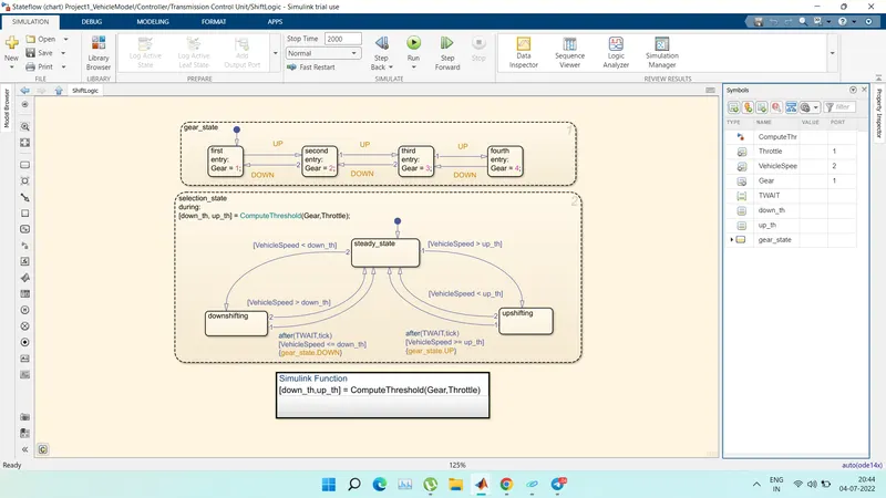
fig- Shift logic unit
- Electric motor control unit
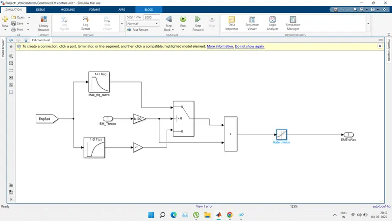
fig-Electric motor control unit
- Powertrain
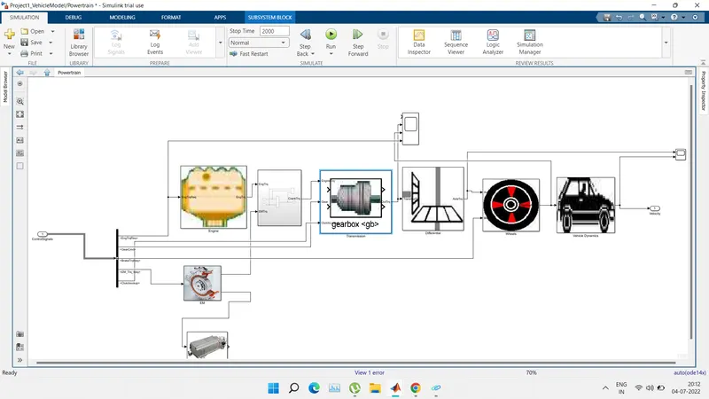
fig-Powertrain
- Engine block diagram
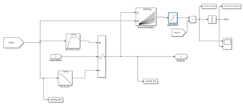
fig-engine block diagram
- Lookup table data
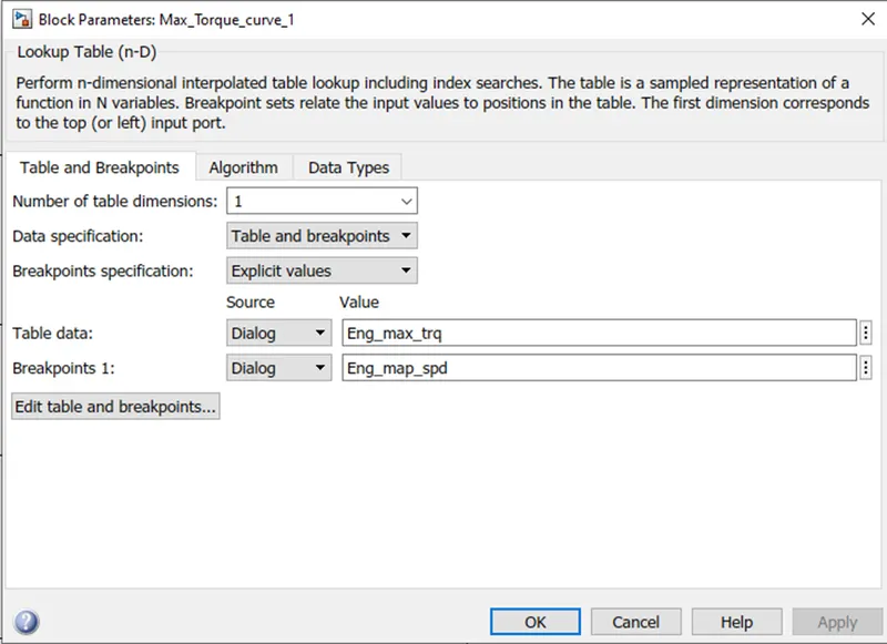
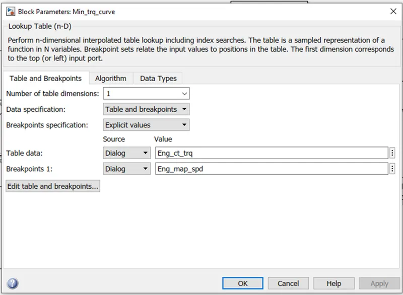
fig-Lookup table
In this model we used map based model to model the fuel consumption of engine. It is based on maximum Torque and minimum torque from the controller, and then it saturated torque and give output then saturated torque and speed map give fuel consumption takes the speed and torque then the output goes into saturated then its integrated.
- Electric motor
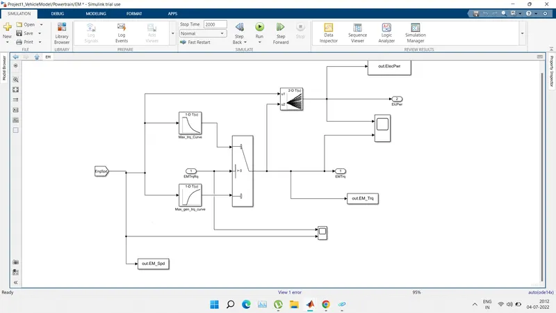
fig-Electric motor
synchronous. There are two types of AC electric motor used to create traction for an electric vehicle: asynchronous (aka induction) and synchronous. In an asynchronous, or induction, motor, the rotor is pulled into a spin, constantly trying to “catch up” with the rotating magnetic field created by the stator.
- Energy storage system
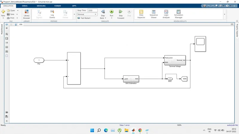
Batteries are the most common chemical energy storage systems in EVs. Lithium ion batteries are currently the dominant battery system employed in EVs. They have been an attractive choice for electric vehicles because they exhibit a high energy density and a long life cycle
- Transmission system
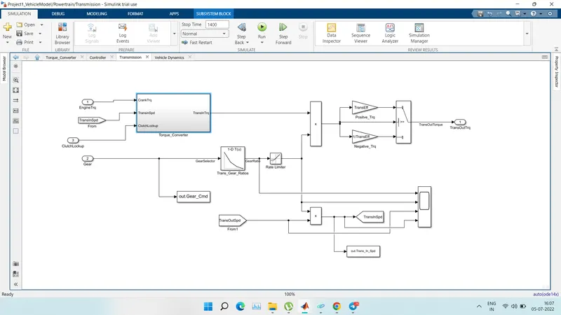
fig- Transmission sytem
A HEV is driven by an ICE in combination with one or more electric motors. A battery package is connected to the motors as a secondary system to provide power to them. Reducing the FC of a HEV is equivalent to improving the efficiency of the HEV powertrain system, especially the working efficiency of the ICE
- Differential
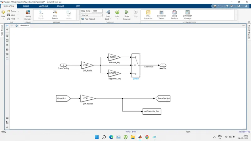
fg- Differential
- vehicle dynamics
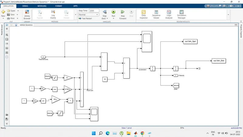
fig-Vehicle dynamics
The conventional power train model is validated using experimental test data confirming accurate emulation of dynamic components of the pre-hybridized vehicle. In addition, the development of dynamic series and parallel hybrid electric vehicle (HEV) powertrain models and corresponding coordinated control laws are described. A discussion of the key issues associated with coordinated control law development is provided. Simulations of the dynamic behavior of two types of series HEVs.
- The following is the matlab programme for various plots and results
%%%%%%%%%%%%%%%%%%%%%%%%%%%%%%%%%%%%%%%%%%%%%%%%%%%%%%%%%%%%%%%%%%%%%
%% Skill-Lync -> Hybrid Drives Development
% Project 1 - Conventional Vehicle Model
% By - Ullekh Gambhira

% Description:
% The following file is to used with the Initialization file and Simulink
% results for post-processing of the data.
% The file is incomplete, has some examples of how the data is imported
% into a readable format, data analysis and plotting examples.
% Based on the project task, use commands in a similar format as given
% below, to analyse the data and generate required plots.
% You can change variable names if desired

%% Post-Processing File
%  File for post-processing the Conventional vehicle simulation model data

%% Renaming variables
Time = out.tout;
Acc_Pdl = out.Acc_Pdl;          % Accelerator pedal [%]
Brk_Pdl = out.Brk_Pdl;          % Brake pedal [%]
Gear_Cmd = out.Gear_Cmd;        % Transmission gear
Trans_In_Spd = out.Trans_In_Spd*30/pi;  % Transmission input speed [rpm]
Trans_Out_Spd = out.Trans_Out_Spd*30/pi;% Transmission output speed [rpm]
Eng_Trq = out.Eng_Trq;          % Engine brake torque [Nm]
Eng_Spd = out.Eng_Spd*30/pi;    % Engine speed [rpm]
Eng_Fuel_Consump = out.Eng_Fuel_Consumption;    % Engine fuel consumption [g]
Veh_Dist = out.Veh_Dist/1000;   % Distance traveled by vehicle [km]
Veh_Spd = out.Veh_Spd*18/5;     % Vehicle speed [kmph]
Eng_Fuel_Rate=out.Eng_Fuel_Rate


%% Data Analysis
Eng_Pwr = Eng_Spd.*pi/30.*Eng_Trq/1000;   % Engine brake power [kW]
rho_petrol = 0.7197;                    % Density of petrol [kg/L]
kmpl = Veh_Dist(end)/(Eng_Fuel_Consump(end)/1000/rho_petrol);    % Fuel economy [kmpl]


%% Plotting vehicle characteristics time trace
figure(1)
subplot(3,1,1)
hold on
grid on
plot(Time, Acc_Pdl, 'linewidth', 1, 'Color', 'black');
plot(Time, Brk_Pdl, 'linewidth', 1, 'Color', 'red');
ylabel('Pedal [%]')
xlim([0, Time(end)]);
legend('Accel','Brake');

subplot(3,1,2)


plot(Time, Trans_In_Spd, 'linewidth', 1, 'Color', 'black');
plot(Time, Trans_Out_Spd, 'linewidth', 1, 'Color', 'red');
ylabel('Speed [rpm]')
xlim([0, Time(end)]);
ylim([0, 6000]);
legend('Trans Input','Trans Output');
subplot(3,1,3)
hold on
grid on
plot(Time, Gear_Cmd, 'linewidth', 1, 'Color', 'black');
xlim([0, Time(end)]);
xlabel('Time [s]');
ylabel('Gear');


%% Plotting engine operating points on engine fuel map
figure(2)
hold on
grid on
title('Engine Operating Points','fontsize',12);
p1=plot(Eng_map_spd*30/pi,Eng_max_trq,'linewidth',2,'color','r');
p2=line([Eng_map_spd(end)*30/pi Eng_map_spd(end)*30/pi],[0 Eng_max_trq(end)]);
set(p2,'linewidth',1,'linestyle','--','color','k');
p3=line([Eng_map_spd(1)*30/pi Eng_map_spd(1)*30/pi],[0 Eng_max_trq(1)]);
set(p3,'linewidth',1,'linestyle','--','color','k');
[c,h] = contour(Eng_map_spd'*30/pi,Eng_map_trq,Eng_fuel_map');
clabel(c,h);
xlabel('Engine Speed [rpm]');
ylabel('Engine Torque [Nm]');
title('Engine Fuel Consumption Map [g/s]');
p4 = plot(Eng_Spd,Eng_Trq,'.','color','k');
legend([p1 p4],{'Max Curve','Operating Points'});
axis([Eng_map_spd(1)*30/pi Eng_map_spd(end)*30/pi 0 Eng_map_trq(end)]);


figure(3)
subplot(2,2,1)

plot(Time, Eng_Trq, 'linewidth', 1, 'Color', 'black');
xlabel('Time');
ylabel('Eng Torque');
hold on
grid on
legend('Eng Trq');


subplot(2,2,2)
plot(Time, Eng_Pwr, 'linewidth', 1, 'Color', 'blue');
xlabel('Time');
ylabel('Eng Power');
hold on
grid on
legend('Eng Pwr');


subplot(2,2,3)
plot(Time, Eng_Fuel_Rate, 'linewidth', 1, 'Color', 'red');
xlabel('Time');
ylabel('Eng Fuel Rate');
hold on
grid on
legend('Eng Fuel_Rate');

subplot(2,2,4)
plot(Time, Eng_Fuel_Consump, 'linewidth', 1, 'Color', 'Green');
xlabel('Time');
ylabel('Eng fuel consumption');
hold on
grid on
legend('Eng Fuel_Consump');

figure(4)

subplot(3,1,1)
plot(Time, out.ElecPwr, 'linewidth',1,'color', 'black')

xlabel('Time [s]')
ylabel('Power [W]')
legend('Electric Motor Power ')
grid on

subplot(3,1,2)

plot(Time,out.EM_Trq,'LineWidth',1,'Color','blue');
xlabel('Time [s]')
ylabel(' Torque [Nm]')
legend('Electric Motor Torque')
grid on

subplot(3,1,3)
plot (Time, out.EM_Spd, 'linewidth',1, 'color', 'red');
xlabel('Time [s]')
ylabel('Speed [Rpm]')
legend('Electrical Motor Speed')
grid on


%Plotting EM Operating Points on motor input power Map

figure('Name', 'Electric Motor Operating Points');
hold on
grid on
title('Electric Motor Operating Points', 'fontsize',12);
pl=plot (EM_map_spd*30/pi, EM_max_trq, 'LineWidth',2, 'color', 'r');
p2=line([EM_map_spd(end)*30/pi EM_map_spd(end)*30/pi], [0 EM_max_trq(end)]);
set(p3,'linewidth',1,'linestyle','--','color','k');
p3=line([EM_map_spd(1)*38/pi EM_map_spd(1)*30/pi], [e EM_max_tra(1)]);
set(p3,linewidth,1, linestyle', 'color','k');
[c,h]= contour (EM_map_spd +30/pi, EM_map_trq, EM_inpwr_map');
clabel(C,h); xlabel('Motor Speed [rpm]');
ylabel('Motor Torque')
legend([p1 p3],{'Max Curve','Operating Points'});
axis([EM_map_spd(1)*30/pi EM_map_spd(end)*30/pi 0 EM_map_trq(end)]);
- for HWFET and UDDS cycle we have got the following output
Fuel Economy Numbers for project 2
S.No
Drive cycle
Fuel Economy Number (KMpl)
UDDS
15.0773
2
HWFET 17.1613
As we see the fuel economy is high in HWFET compared to UDDS. It is because in urban driving the vehicle encounters more traffic and it has to stop for fever distance and it consumes more fuel at the starting. In HWFET the vehicle encounters no traffic and it moves without use of too much braking so it will have more fuel economy number.
Comparing with fuel economy numbers for project 1
S.No
Drive cycle
Fuel Economy Number (KMpl)
1
UDDS
14.209
2
HWEET
16.503
As we see the fuel economy numbers for project 2 are bit higher when compared to project 1 because of implementing the electric motor as it is P1 hybrid it may not have much variation in the fuel economy but as we implement other architechture it will increase by huge amount.
- b. Plot the time trace for engine, transmission input, transmission output and wheel speed on one plot. for UDDS
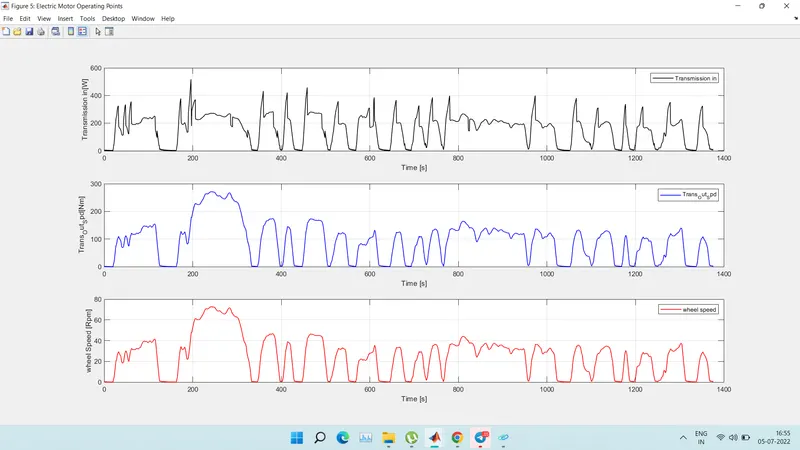
fig-time trace for engine, transmission input, transmission output and wheel speed
- HWFET
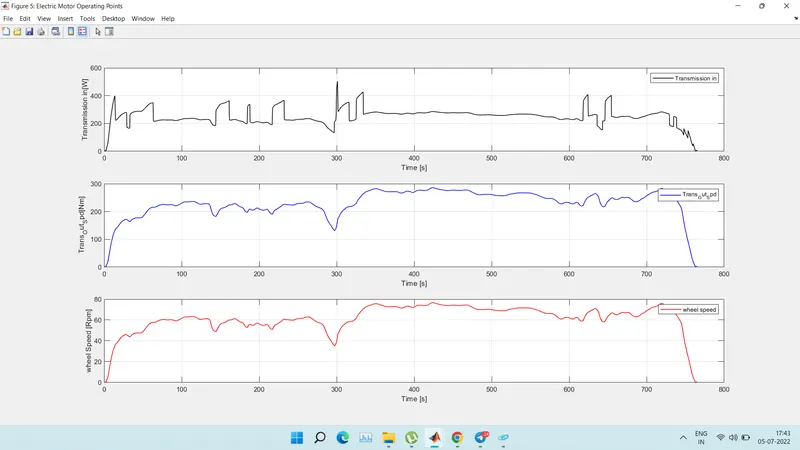
fig-time trace for engine, transmission input, transmission output and wheel speed
- c. Plot engine torque, engine power, fuel rate and fuel consumption using subplots UDDS
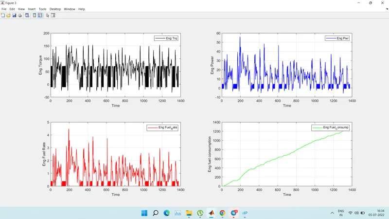
fig-engine torque, engine power, fuel rate and fuel consumption
- HWFET
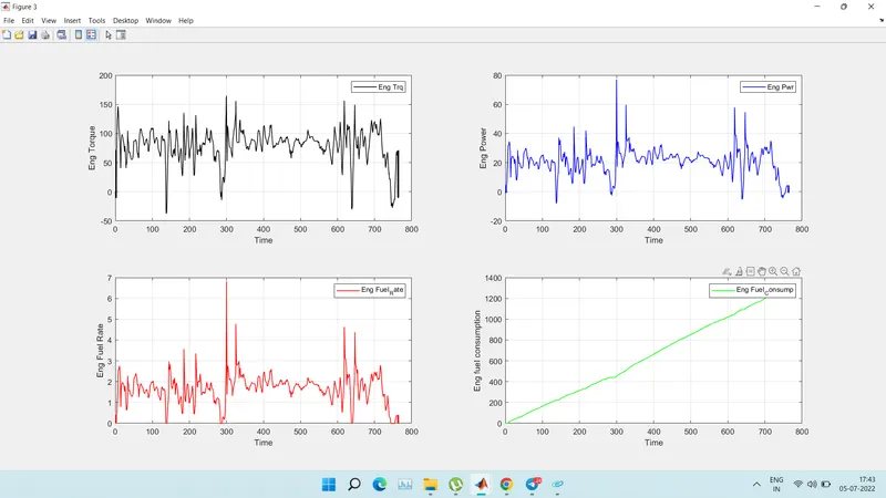
fig-engine torque, engine power, fuel rate and fuel consumption
Vehicle cosumed more power in UDDS drive ccycle bacause in urban area the vehicle require many starts and stops so it required more power compred to HWFET. Engine is high in UDDS drive cycle compred to HWFET drive cycle because the starting from rest the vehicle requires more torque to overcome the static friction. The fuel rate is high in HWFET drive cycle compared to UDDS drive cycle because it will be in continues movement so it consumes more fuel.
The fuel economy is high in HWFET because in UDDS cycle many starts and stops so more fuel cosumes and the engine is in idle postion.
- d. Plot accelerator and brake pedal, gear command, vehicle desired and actual speed, vehicle distance using subplots.
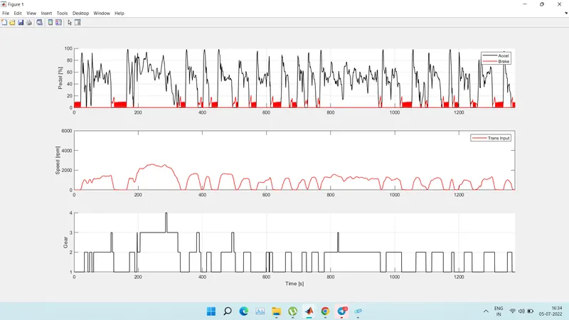
fig-accelerator and brake pedal, gear command, vehicle desired and actual speed, vehicle distance
- HWFET
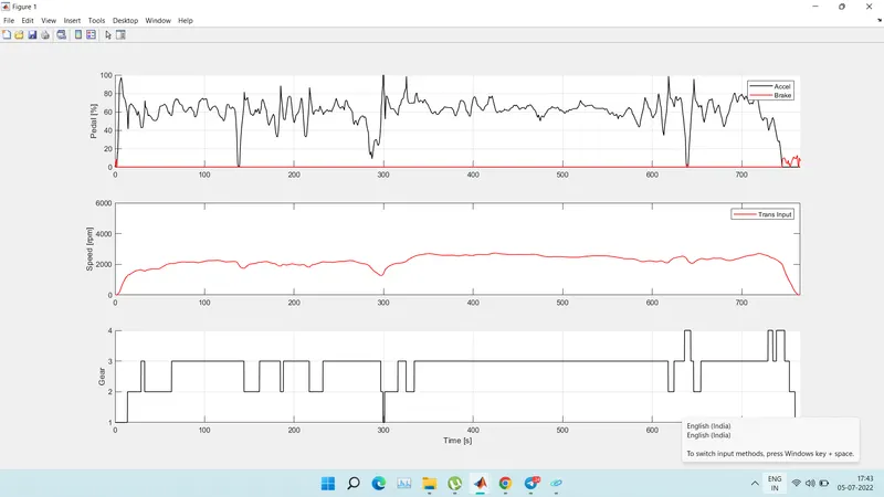
fig-accelerator and brake pedal, gear command, vehicle desired and actual speed, vehicle distance
In UDDS The acceleration and brake pedal have more fluctuations because of frequent starts and stops. but in HWFET the brake pedal fluctuations are almost near to the zero line as there will be no frequent stops.
In UDDS cycle mostly runs on 1st and 2nd gears and the 3rd and 4th gears are rarely useas it does not achieve high speed inn that traffic. In The HWFET cycle the vehicle mostly runn in 3rd and 4th gears as it will moving at high speeds.
- e. Plot the engine operating points on the engine fuel map.
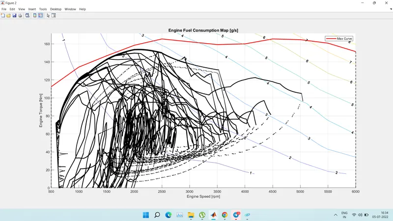
fig-engine operating points
- HWFET
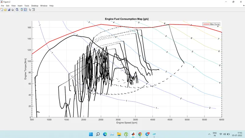
fig-engine operating points
- f. Plot motor speed, torque, motor input power using subplots.
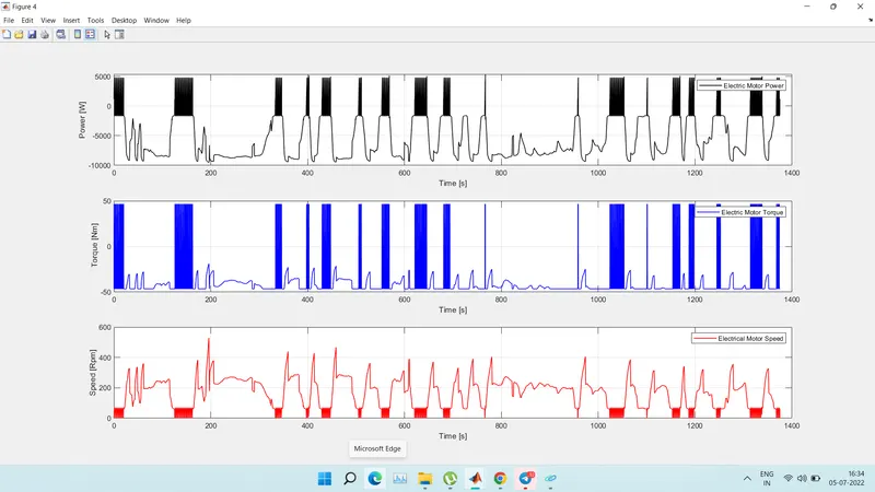
fig-motor speed, torque, motor input power
HWFET
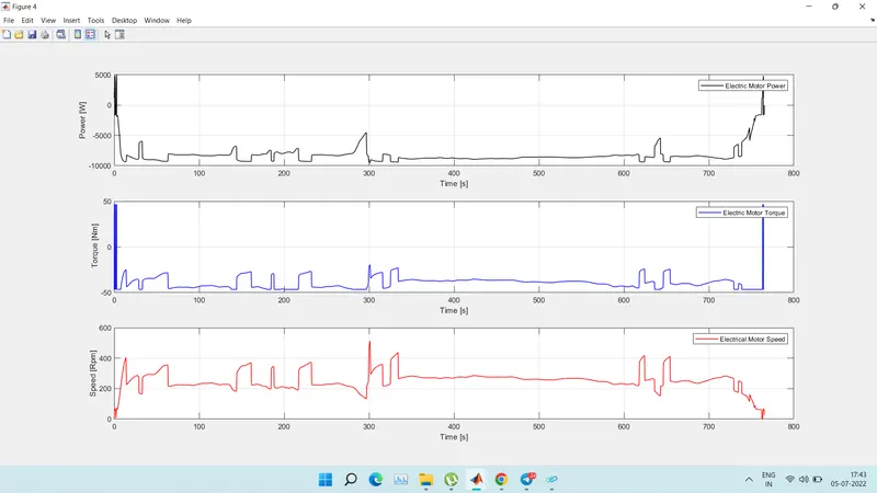
fig-motor speed, torque, motor input power
The fluctuations will be more in UDDS cycle compared to HWFET cycle because UDDS has many starts and stops due to traffic as the purpose of motor in Pt hybrid is initiation of crank rotation and they are more in UDDS cycle when compared HWFET cycle. If the purpose of the motor is to provide traction then both the cycles would have more flyctuations. We can observe that the motor power and torque are very high in HWFET at the start and they are almost zero after few seconds but in UDDS it has continuod fluctuations this is because of frequent braking in UDDS,
g. Plot pack voltage, current and SoC using subplots.
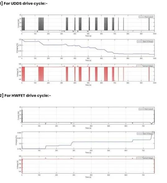
fig- Plot pack voltage, current and SoC
The pack voltage and current will have more fluctuations in UDDS as compared to HWFET cycle because of the frequent start and stops throughout the drive and the battery has to provide the energgy everytime when the car is starting from the idle position
SOC decreased in the UDDS cycle wrt time but it has increased in HWFET cycle. It is because in UDDS we have frequent start and stops and battery has to provide the energy has evertytime when the carls starting from the Idle position and the SOC decreases but in HWFET cycle The Vehicle will be moving continuously without braking frequently and the alternator is utilised to transfer some engine power to the battery through motor so SOC increase in the HWFET cycle
- h. Plot the motor operating points on the motor input power map, with the motor max
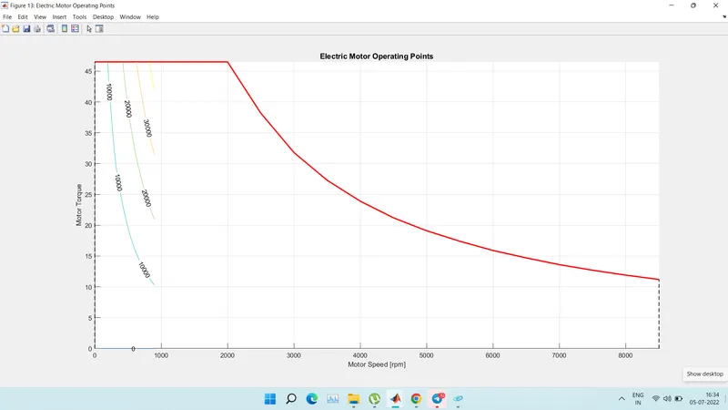
fig-motor operating points on the motor input power map, with the motor max
- HWFET
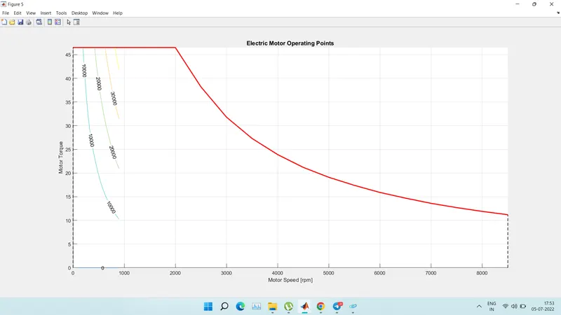
fig-motor operating points on the motor input power map, with the motor max
- Conclusion
The various performance of characteristics and operating points of UDDS drive cycle and HWFET drive cycle are analysed and the graphs are plotted • Time trace for engine, Transmission input, Transmission output and wheelspeed with respect to time. Engine torque, Engine power, Fuel rate and Fuel consumption with respect to time. • Accelerator and brake pedal, gear command and vehicle desired, actual speed, vehicle distance with respect to time. Engine operating points on the engine fuel map with respect to time. Motor speed, Torque, Motor Input power with respect to time. Pack voltage, Current and State of charging with respect to time. • The motor operating points on the motor input power map with respect to time. and also it comparing with HWFET drive cycle and their numbers also compared.