Project 2

Description:
As discussed in Lecture 11, Project 2 deals with the development of a forward energy-based fuel consumption model of a P1 hybrid vehicle. This model is based on the conventional vehicle model from Project 1.

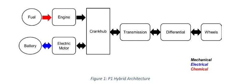
The main goal of this project is to understand the functionality of a P1 hybrid and be able to model it.

Honda Insight motor and battery are considered for this project. Data is taken from ADVISOR data base developed by NREL, USA. Data provided in the project files.

“Project2_InitFile.m” is a Matlab script used to load all the variables required for running the Simulink model and for post-processing. The drive cycle selection is also done here. Before running the Simulink vehicle model, run this initialization script.

Task:

The task of this project is to quantify the improvement in fuel economy numbers for the hybrid vehicle (kmpl), compared to the conventional vehicle, on the urban cycle (UDDS) and highway cycle (HWFET). Also, to analyze and understand the vehicle operating points in terms of engine and motor speed, torque, transmission speeds, pedal positions, gear, distance traveled, battery voltage, current, SoC etc.

To do that, the following steps need to be followed:

1) Load the Project2 folder as the Current Folder in Matlab.
2) Run the “Project2_InitFile.m” Matlab script.
3) Copy the Conventional vehicle Simulink model created for Project 1 in this folder. Figure 1: P1 Hybrid ArchitectureHybrid Drives Development
4) Modify this model into a hybrid vehicle model. The lecture presentations can be used as reference. Battery and Supervisory controller models developed in the assignments can be reused.
5) Add additional ‘To Workspace’ blocks for transferring the desired Simulink vehicle data into the Matlab workspace.
6) Simulate the hybrid model on the desired drive cycles.
7) Write a project report that contains the following:
a. Tabulate the fuel economy numbers (kmpl) for UDDS and HWFET cycle. Compare these numbers with the baseline numbers for conventional vehicle model from Project 1.
b. Plot the time trace for engine, transmission input, transmission output and wheel speed on one plot.
c. Plot engine torque, engine power, fuel rate and fuel consumption using subplots.
d. Plot accelerator and brake pedal, gear command, vehicle desired and actual speed, vehicle distance using subplots.
e. Plot the engine operating points on the engine fuel map.
f. Plot motor speed, torque, motor input power using subplots.
g. Plot pack voltage, current and SoC using subplots.
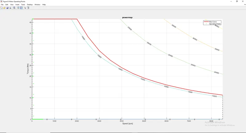
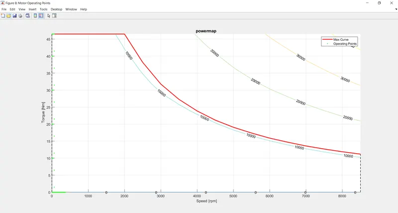
h. Plot the motor operating points on the motor input power map, with the motor max motoring and generating torque curves.
i. Write down appropriate brief comments on each of these plots, describing the vehicle behavior throughout the drive cycle.
j. Generate the plots for both drive cycles

Ans )

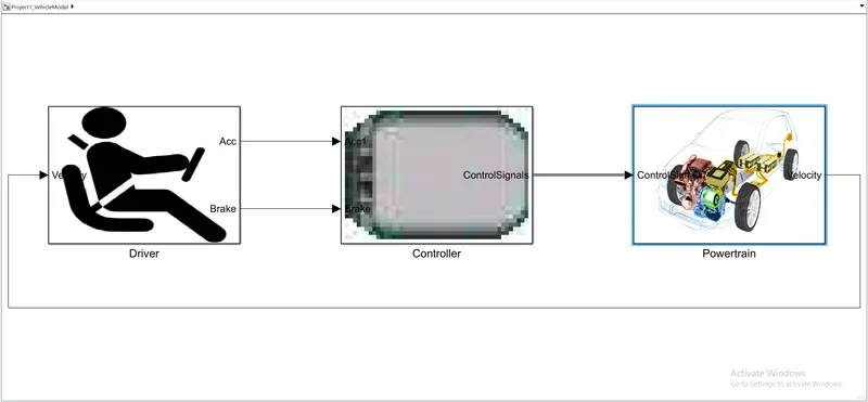
Driver block

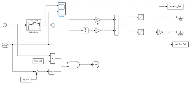
Controller

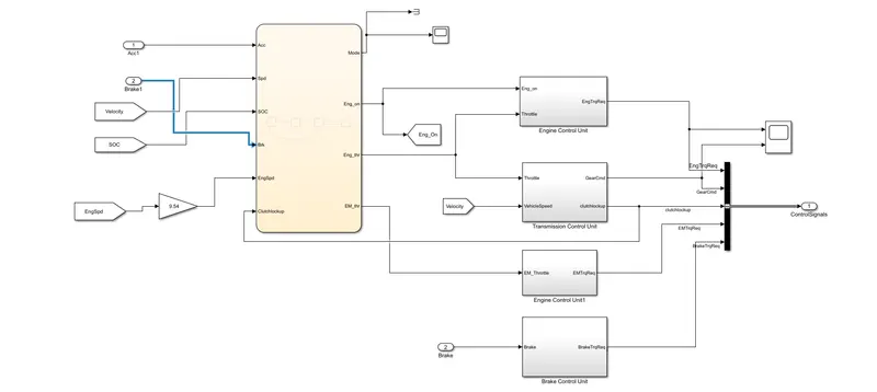
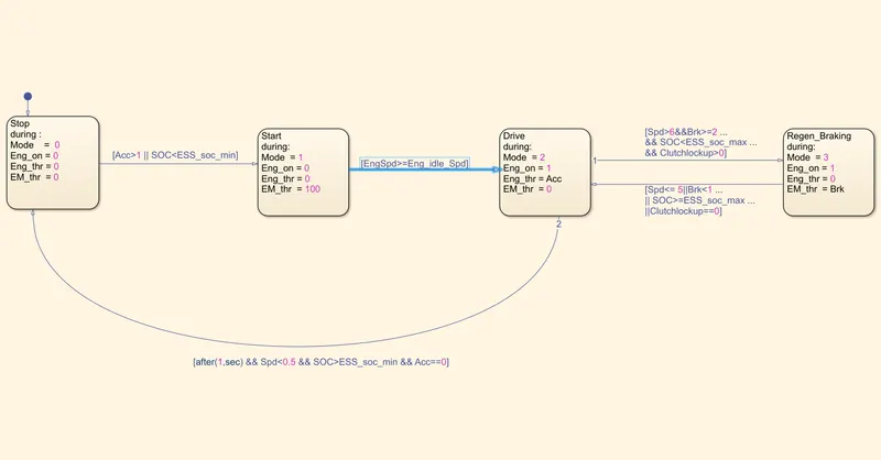
• Open the Simulink work area and type 'outline' and the Stateflow diagram opens up
• Make an underlying block
• The underlying block addresses the 'stop' condition, in which the motor is off, motor and engine choke conditions are zero
• Make a second block that addresses mode-1. In this, the electric engine choke is simply used to give the necessary force and capacity to the vehicle. The motor is off and motor choke condition is zero
  States 1&2 are associated utilizing the connections for example it moves from state-1 to state-2 when speed increase is short of what one or SOC is not exactly the base SOC
  
• State-3 addresses mode-2 for example motor is on and the motor choke is likewise having some certain worth from the driver however the electric engine choke is zero. It changes from state-2 to state-3 when motor speed is more noteworthy than or equivalent to the motor stand-by speed
  
• State-4 addresses regenerative slowing down which is mode-3. In this express, the motor is on however the motor choke is having no contribution from the driver, though the electric engine gets the negative power i.e because of the slowing down
  
• State-4 is accomplished from the state-3 when SOC is not exactly most extreme SOC or when grip lockup is more prominent than nothingState-4 actions to state-3 when SOC is more noteworthy than or equivalent to greatest SOC or when grip lockup is equivalent to nothing
  
• There is an opportunity of state-3 moving to state-1 when SOC is more prominent than least SOC and speed increase is zero
• The data sources given to the graph are speed increase, brake, motor speed, vehicle speed, SOC, and grip lockup
  
• The results that we get from the diagram are mode, motor condition (on or off), motor choke condition, and electric engine choke condition

Engine Control Unit

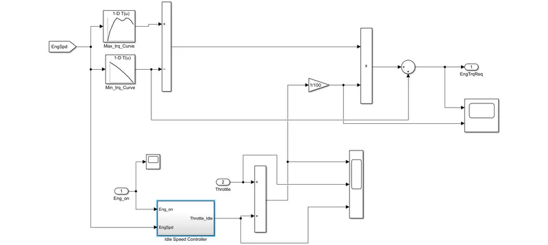
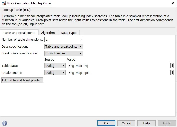
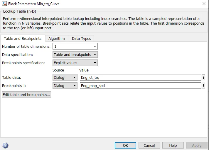
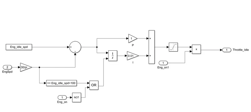
Idle speed controller (ECU)

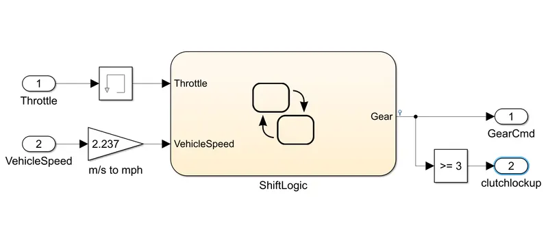
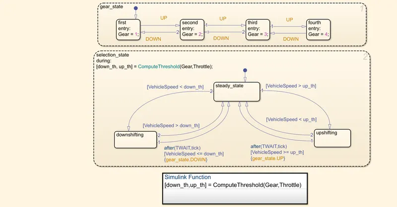
Transmission control unit

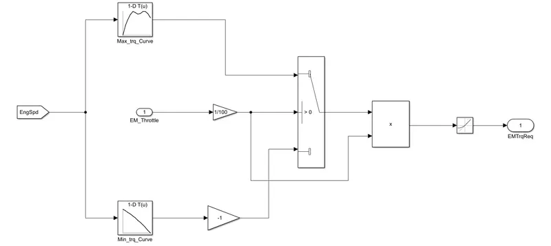
EM Control Unit

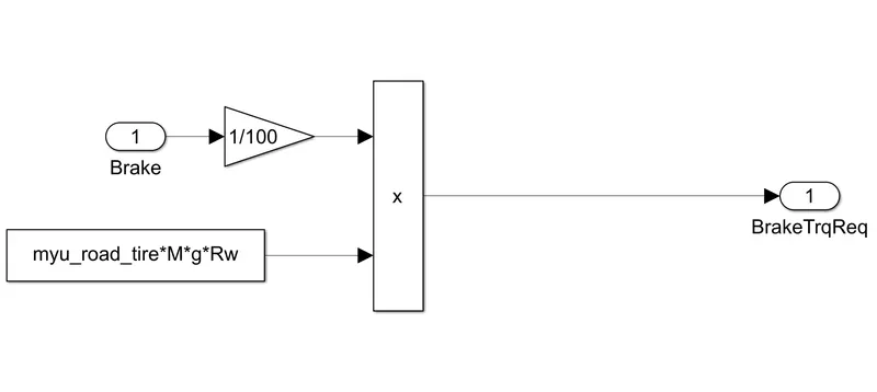
Brake control Unit

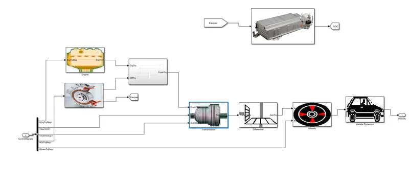
Power Train

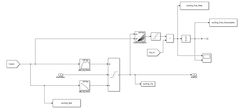
Engine block diagram

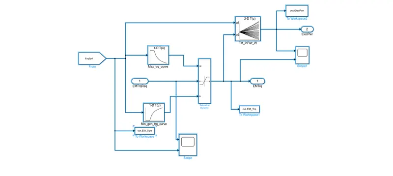
Electric Motor

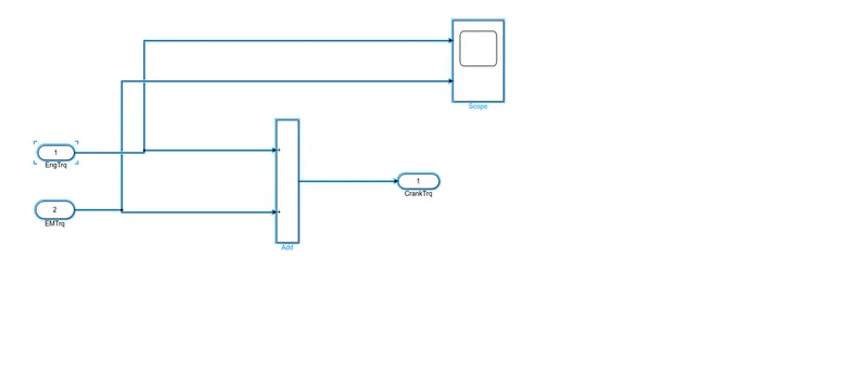
Crank Torque Subsystem.

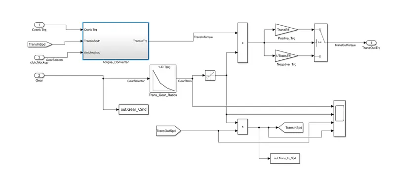
Transmission system

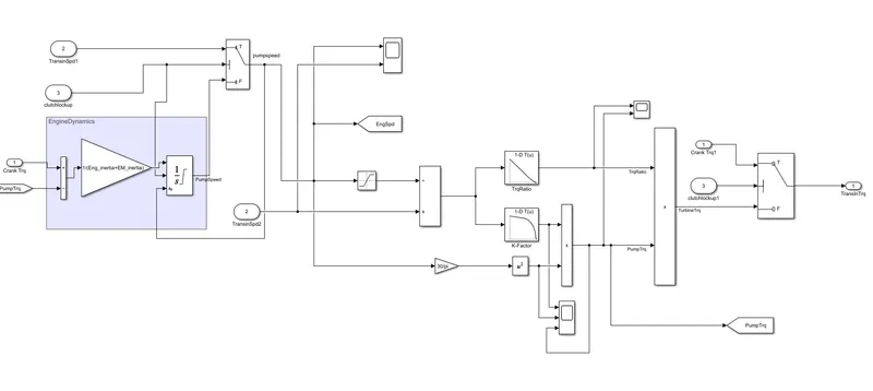
The torque converter in transmission

Wheels

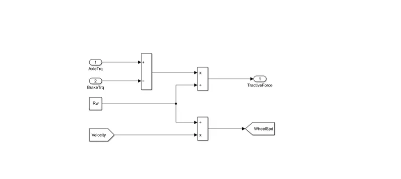
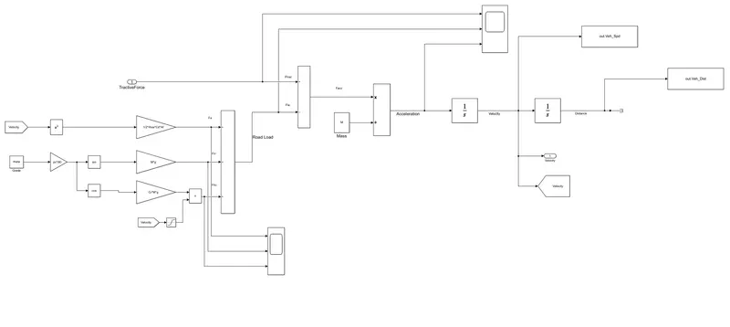
Vehicle Dynamics

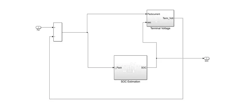
Energy storage system

a) Fuel Economy numbers (kmpl) for UDDS

%%%%%%%%%%%%%%%%%%%%%%%%%%%%%%%%%%%%%%%%%%%%%%%%%%%%%%%%%%%%%%%%%%%%%
%% Skill-Lync -> Hybrid Drives Development
% Project 1 - Conventional Vehicle Model
% By - Ullekh Gambhira 

% Description:

%% Initialization File
% Initialization file for loading the variables for the Conventional vehicle simulation model

%% Vehicle Parameters
M = 1500;       % Vehicle weight [kg]
Cr = 0.015;     % Rolling resistance coefficient
Rw = 0.35;      % Rolling radius [m]
Cd = 0.33;      % Drag coefficient
Af = 2;         % Frontal area [m2]
rhoa = 1.225;   % Air density [kg/m3]
Vwind = 0;      % Wind velocity [kmph]
g = 9.81;       % Gravitational acceleration [m/s2]
theta = 0;      % Slope [deg]
myu_road_tire = 1; % Coefficient of friction between tire - road interface

%% Powertrain Parameters 
FDR = 3.73;                         % Final Drive Ratio / Diff Ratio
DiffEff = 0.99;                     % Differential efficiency (assumed independent of operating conditions)

NumGear = 4;                        % Number of gears in transmission
TransGear = [1:NumGear];            % Transmission Gears
TransRatio = [3.06, 1.62, 1, 0.7];  % Corresponding Transmission ratios
TransEff = 0.90;                    % Transmission efficiency (assumed independent of operating conditions)

TC_SR = [0, .5, .6, .7, .8, .87, .92, .94, .96, .97, 1];   % Torque Converter Speed Ratio (Matlab default) -> TurbSpd/PumpSpd  
TC_TR = [2.232, 1.5462, 1.4058, 1.2746, 1.1528, 1.0732, 1.0192, 1, 1, 1, 1];   % Torque Converter Torque Ratio (Matlab default) -> TurbTrq/PumpTrq
TC_Cf = 1e-4 * [.72558, .66322, .63463, .59042, .51331, .4144, .29287, .22444, .12186, .04386, 0]; % Torque Converter Capacity Factor (Matlab default) -> PumpTrq/PumpSpd^2 [Nm/rpm^2]

load Vehicle_Data/Engine_data_1_9L_Saturn_95kW
load Vehicle_Data/Trans_Shift_map
load Vehicle_Data/EM_Honda_Insight_10kW
load Vehicle_Data/ESS_NiMH6


ESS_init_soc = 0.8;
ESS_soc_max = 0.9;
ESS_soc_min = 0.6;


%% Driver Parameters
Kp = 10;                    % P gain for driver PI model
Ki = 1;                     % I gain for driver PI model
Drive_Cycle_Select = 1;     % Drive cycle selection

% Drive cycle values in m/s

if Drive_Cycle_Select == 1
    load DriveCycles/UDDS;
    
elseif Drive_Cycle_Select == 2
    load DriveCycles/HWFET;
    
elseif Drive_Cycle_Select == 3
    load DriveCycles/FTP;
    
elseif Drive_Cycle_Select == 4
    load DriveCycles/US06;
    
elseif Drive_Cycle_Select == 5
    load DriveCycles/NEDC;
    
elseif Drive_Cycle_Select == 6
    load DriveCycles/WLTP;
 
end

time_end = cyc_time(end);
vel_end = cyc_vel(end);

%%%%%%%%%%%%%%%%%%%%%%%%%%%%%%%%%%%%%%%%%%%%%%%%%%%%%%%%%%%%%%%%%%%%%
%% Skill-Lync -> Hybrid Drives Development
% Project 2 - hybrid Vehicle Model
% By - Ullekh Gambhira 

% Description:
% The following file is to used with the Initialization file and Simulink
% results for post-processing of the data.
% The file is incomplete, has some examples of how the data is imported
% into a readable format, data analysis and plotting examples.
% Based on the project task, use commands in a similar format as given
% below, to analyse the data and generate required plots.
% You can change variable names if desired

%% Post-Processing File
%  File for post-processing the Conventional vehicle simulation model data

%% Renaming variables
Time = out.tout;
Acc_Pdl = out.Acc_Pdl;          % Accelerator pedal [%]
Brk_Pdl = out.Brk_Pdl;          % Brake pedal [%]
Gear_Cmd = out.Gear_Cmd;        % Transmission gear
Trans_In_Spd = out.Trans_In_Spd*30/pi;  % Transmission input speed [rpm]
Trans_Out_Spd = out.Trans_Out_Spd*30/pi;% Transmission output speed [rpm]
Eng_Trq = out.Eng_Trq;          % Engine brake torque [Nm]
Eng_Spd = out.Eng_Spd*30/pi;    % Engine speed [rpm]
Eng_Fuel_Consump = out.Eng_Fuel_Consumption;    % Engine fuel consumption [g]
Veh_Dist = out.Veh_Dist/1000;   % Distance traveled by vehicle [km]
Veh_Spd = out.Veh_Spd*18/5;     % Vehicle speed [kmph]
Eng_Fuel_Rate=out.Eng_Fuel_Rate;%Engine fuel rate%

%% Data Analysis
Eng_Pwr = Eng_Spd.*pi/30.*Eng_Trq/1000;   % Engine brake power [kW]
rho_petrol = 0.7197;                    % Density of petrol [kg/L]
kmpl = Veh_Dist(end)/(Eng_Fuel_Consump(end)/1000/rho_petrol);    % Fuel economy [kmpl] 


%% Plotting vehicle characteristics time trace
figure(1)
subplot(3,1,1)
hold on
grid on
plot(Time, Eng_Spd, 'linewidth', 1, 'Color', 'black');
ylabel('Eng_Spd')
xlim([0, Time(end)]);
legend('Eng_Spd');
subplot(3,1,2)
hold on
grid on
plot(Time, Trans_In_Spd, 'linewidth', 1, 'Color', 'black');
plot(Time, Trans_Out_Spd, 'linewidth', 1, 'Color', 'red');
ylabel('Speed [rpm]')
xlim([0, Time(end)]);
ylim([0, 6000]);
legend('Trans Input','Trans Output');
subplot(3,1,3)
hold on
grid on
plot(Time, Veh_Spd, 'linewidth', 1, 'Color', 'black');
xlim([0, Time(end)]);
xlabel('Time [s]');
ylabel('Vehicle_Speed');
legend('Vehicle_Spd');

figure(2)
subplot(3,1,1)
hold on
grid on
plot(Time, Eng_Trq, 'linewidth', 1, 'Color', 'red');
ylabel('Engine Torque [Nm]')
xlim([0, Time(end)]);
legend('Eng Trq');
subplot(3,1,2)
hold on
grid on
plot(Time, Eng_Pwr, 'linewidth', 1, 'Color', 'red');
ylabel('Engine Power [KW]')
xlim([0, Time(end)]);
legend('Power');
subplot(3,1,3)
hold on
grid on
plot(Time,Eng_Fuel_Consump , 'linewidth', 1, 'Color', 'green');
xlim([0, Time(end)]);
xlabel('Time [s]');
ylabel('Fuel Consumption');

figure(3)
subplot(3,1,1)
hold on
grid on
plot(Time, Eng_Trq, 'linewidth', 1, 'Color', 'red');
ylabel('Engine Torque [Nm]')
xlim([0, Time(end)]);
legend('Eng Trq');
subplot(3,1,2)
hold on
grid on
plot(Time, Eng_Pwr, 'linewidth', 1, 'Color', 'red');
ylabel('Engine Power [KW]')
xlim([0, Time(end)]);
legend('Power');
subplot(3,1,3)
hold on
grid on
plot(Time,Eng_Fuel_Rate , 'linewidth', 1, 'Color', 'black');
xlim([0, Time(end)]);
xlabel('Time [s]');
ylabel('Eng_Fuel_Rate');

figure(4)
subplot(3,1,1)
hold on
grid on
plot(Time, Acc_Pdl, 'linewidth', 1, 'Color', 'red');
plot(Time, Brk_Pdl, 'linewidth', 1, 'Color', 'blue');
ylabel('Pedal')
xlim([0, Time(end)]);
legend('Acc_Pdl','Brk_pdl');
subplot(3,1,2)
hold on
grid on
plot(Time, Gear_Cmd, 'linewidth', 1, 'Color', 'red');
ylabel('Gear')
xlim([0, Time(end)]);
legend('Gear_Cmd');
subplot(3,1,3)
hold on
grid on
plot(Time,Veh_Spd, 'linewidth', 1, 'Color', 'black');
xlim([0, Time(end)]);
xlabel('Time [s]');
ylabel('Veh_Spd');
legend('Veh_Spd');

figure(5)
subplot(3,1,1)
hold on
grid on
plot(Time,out.EM_Trq,'linewidth',1,'color','red');
ylabel('Motor Torque[Nm]');
xlim([0,Time(end)]);
legend('Motor Trq');
subplot(3,1,2)
hold on
grid on
plot(Time,out.ElecPwr,'linewidth',1,'color','red');
ylabel('motor power (kw)');
xlim([0,Time(end)]);
legend('Motor power');
subplot(3,1,3)
hold on
grid on
plot(Time, out.EM_Spd, 'linewidth',1,'color','green');
xlim([0,Time(end)]);
xlabel('Time(s)');
ylabel('motor speed');

figure(6)
subplot(3,1,1)
hold on
grid on
plot(Time, out.term_volt,'linewidth',1,'color','green');
ylabel('Voltage(V)');
xlim([0,Time(end)]);
legend('voltage');
subplot(3,1,2)
hold on
grid on
plot(Time,out.soc,'linewidth',1,'color','red');
ylabel('SOC');
xlim([0,Time(end)]);
legend('SOC %')
subplot(3,1,3)
hold on
grid on
plot(Time,out.pack_Current,'linewidth',1,'color','blue');
ylabel('SOC');
xlim([0,Time(end)]);
xlabel('Time(s)');
ylabel('pack_current');


%% Plotting engine operating points on engine fuel map
figure('Name','Engine Operating Points');
hold on
grid on
title('Engine Operating Points','fontsize',12);
p1=plot(Eng_map_spd*30/pi,Eng_max_trq,'linewidth',2,'color','r');
p2=line([Eng_map_spd(end)*30/pi Eng_map_spd(end)*30/pi],[0 Eng_max_trq(end)]);
set(p2,'linewidth',1,'linestyle','--','color','k');
p3=line([Eng_map_spd(1)*30/pi Eng_map_spd(1)*30/pi],[0 Eng_max_trq(1)]);
set(p3,'linewidth',1,'linestyle','--','color','k');
[c,h] = contour(Eng_map_spd'*30/pi,Eng_map_trq,Eng_fuel_map');
clabel(c,h);
xlabel('Engine Speed [rpm]');
ylabel('Engine Torque [Nm]');
title('Engine Fuel Consumption Map [g/s]');
p4 = plot(Eng_Spd,Eng_Trq,'.','color','k');
legend([p1 p4],{'Max Curve','Operating Points'});
axis([Eng_map_spd(1)*30/pi Eng_map_spd(end)*30/pi 0 Eng_map_trq(end)]);

%% Plotting motor operating points on engine fuel map
figure('Name','Motor Operating Points');
hold on
grid on
title('Motor Operating Points','fontsize',12);
p1=plot(EM_map_spd*30/pi,EM_max_trq,'linewidth',2,'color','r');
p2=line([EM_map_spd(end)*30/pi EM_map_spd(end)*30/pi],[0 EM_max_trq(end)]);
set(p2,'linewidth',1,'linestyle','--','color','k');
p3=line([EM_map_spd(1)*30/pi EM_map_spd(1)*30/pi],[0 EM_max_trq(1)]);
set(p3,'linewidth',1,'linestyle','--','color','k');
[c,h] = contour(EM_map_spd'*30/pi,EM_map_trq,EM_inpwr_map');
clabel(c,h);
xlabel(' Speed [rpm]');
ylabel(' Torque [Nm]');
title('powermap');
p4 = plot(out.EM_Spd,out.EM_Trq,'.','color','g');
legend([p1 p4],{'Max Curve','Operating Points'});
axis([EM_map_spd(1)*30/pi EM_map_spd(end)*30/pi 0 EM_map_trq(end)]);

fig 1

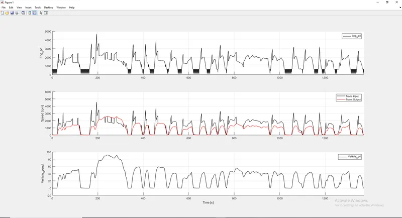
Fig 2

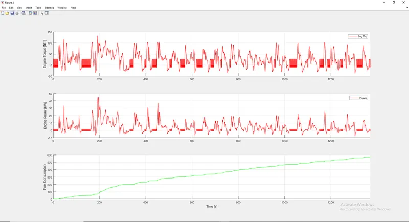
Fig 3

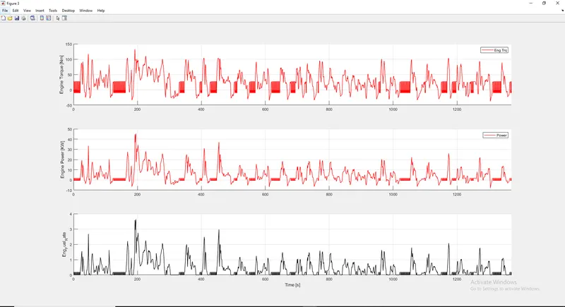
Fig 4

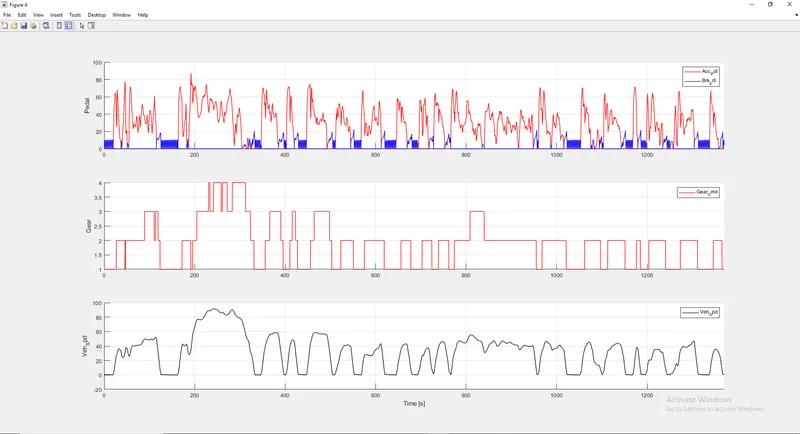
Fig 5

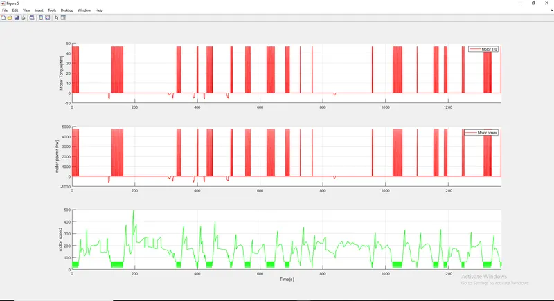
Fig 6

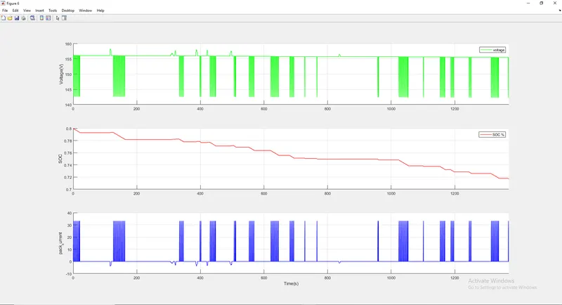
Fig 7

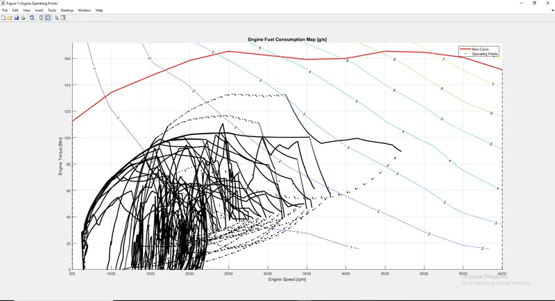
Fig 8

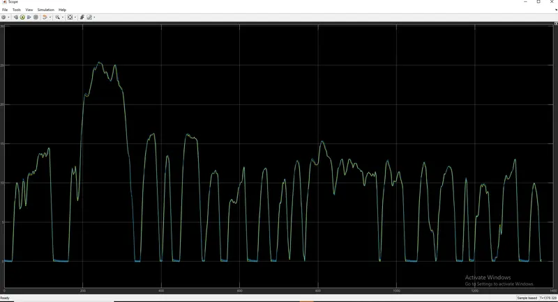
a) Fuel Economy numbers (kmpl) for UDDS =15.1277

• For UDDS, the gas pedal and the brake pedal have more changes due to visit starts and stops. Be that as it may, in HWFET, the brake pedal changes are practically close to the no line as there will be no regular stops
• UDDS cycle for the most part runs on first, second cog wheels, and uses third, fourth cog wheels seldom as it doesn't accomplish high velocities in that rush hour gridlock. In the HWFET cycle, the vehicle for the most part runs on third, fourth cog wheels as it will be moving at high velocities. It utilizes first, second pinion wheels as often as possible while slowing down is required
• Clearly, the vehicle paces will be high in HWFET contrasted with UDDS. UDDS likewise has more changes in the speed because of successive slowing down
  The distance went in the given time will be high in HWFET than UDDS in view of the traffic hindrance in UDDS
• The variances will be more in UDDS cycle contrasted with HWFET cycle on the grounds that, UDDS has many beginnings and stops because of traffic, as the reason for engine in P1 cross breed is commencement of wrench turn and they are more in UDDS cycle when contrasted with HWFET cycle
• On the off chance that the motivation behind the engine is to give foothold, both the cycles would have more variances
• We can obeserve that, the engine power and force are extremely high in HWFET toward the beginning and they are very nearly zero following couple of moments however in UDDS it has persistent vacillations. This is a result of continuous slowing down in UDDS

comparison of pack current , pack pack voltage

• The variations will be similar to that of the motor because, battery is the energy reservoir and it gives the energy for the motor to run
• Pack voltage and current will have more fluctuationsin UDDS as compared to HWFET because of frequent start and stops throughout the drive and battery has to provide the energy everytime when the car is starting from the idle position
• SOC decreased in the UDDS cycle wrt time but it has increased in the HWFET cycle. It is because in UDDS cycle we have frequent start and stops and battery has to provide the energy everytime when the car is starting from the idle position and the SOC decreases. But in HWFET cycle, the vehicle will be moving continuously without braking frequently and the alternator is utilised to transfer some engine power to the battery through motor, so SOC increases in the HWFET cycle

b) Fuel Economy numbers (kmpl) for HWFET

%%%%%%%%%%%%%%%%%%%%%%%%%%%%%%%%%%%%%%%%%%%%%%%%%%%%%%%%%%%%%%%%%%%%%
%% Skill-Lync -> Hybrid Drives Development
% Project 1 - Conventional Vehicle Model
% By - Ullekh Gambhira 

% Description:

%% Initialization File
% Initialization file for loading the variables for the Conventional vehicle simulation model

%% Vehicle Parameters
M = 1500;       % Vehicle weight [kg]
Cr = 0.015;     % Rolling resistance coefficient
Rw = 0.35;      % Rolling radius [m]
Cd = 0.33;      % Drag coefficient
Af = 2;         % Frontal area [m2]
rhoa = 1.225;   % Air density [kg/m3]
Vwind = 0;      % Wind velocity [kmph]
g = 9.81;       % Gravitational acceleration [m/s2]
theta = 0;      % Slope [deg]
myu_road_tire = 1; % Coefficient of friction between tire - road interface

%% Powertrain Parameters 
FDR = 3.73;                         % Final Drive Ratio / Diff Ratio
DiffEff = 0.99;                     % Differential efficiency (assumed independent of operating conditions)

NumGear = 4;                        % Number of gears in transmission
TransGear = [1:NumGear];            % Transmission Gears
TransRatio = [3.06, 1.62, 1, 0.7];  % Corresponding Transmission ratios
TransEff = 0.90;                    % Transmission efficiency (assumed independent of operating conditions)

TC_SR = [0, .5, .6, .7, .8, .87, .92, .94, .96, .97, 1];   % Torque Converter Speed Ratio (Matlab default) -> TurbSpd/PumpSpd  
TC_TR = [2.232, 1.5462, 1.4058, 1.2746, 1.1528, 1.0732, 1.0192, 1, 1, 1, 1];   % Torque Converter Torque Ratio (Matlab default) -> TurbTrq/PumpTrq
TC_Cf = 1e-4 * [.72558, .66322, .63463, .59042, .51331, .4144, .29287, .22444, .12186, .04386, 0]; % Torque Converter Capacity Factor (Matlab default) -> PumpTrq/PumpSpd^2 [Nm/rpm^2]

load Vehicle_Data/Engine_data_1_9L_Saturn_95kW
load Vehicle_Data/Trans_Shift_map
load Vehicle_Data/EM_Honda_Insight_10kW
load Vehicle_Data/ESS_NiMH6


ESS_init_soc = 0.8;
ESS_soc_max = 0.9;
ESS_soc_min = 0.6;


%% Driver Parameters
Kp = 10;                    % P gain for driver PI model
Ki = 1;                     % I gain for driver PI model
Drive_Cycle_Select = 2;     % Drive cycle selection

% Drive cycle values in m/s

if Drive_Cycle_Select == 1
    load DriveCycles/UDDS;
    
elseif Drive_Cycle_Select == 2
    load DriveCycles/HWFET;
    
elseif Drive_Cycle_Select == 3
    load DriveCycles/FTP;
    
elseif Drive_Cycle_Select == 4
    load DriveCycles/US06;
    
elseif Drive_Cycle_Select == 5
    load DriveCycles/NEDC;
    
elseif Drive_Cycle_Select == 6
    load DriveCycles/WLTP;
 
end

time_end = cyc_time(end);
vel_end = cyc_vel(end);

%%%%%%%%%%%%%%%%%%%%%%%%%%%%%%%%%%%%%%%%%%%%%%%%%%%%%%%%%%%%%%%%%%%%%
%% Skill-Lync -> Hybrid Drives Development
% Project 2 - hybrid Vehicle Model
% By - Ullekh Gambhira 

% Description:
% The following file is to used with the Initialization file and Simulink
% results for post-processing of the data.
% The file is incomplete, has some examples of how the data is imported
% into a readable format, data analysis and plotting examples.
% Based on the project task, use commands in a similar format as given
% below, to analyse the data and generate required plots.
% You can change variable names if desired

%% Post-Processing File
%  File for post-processing the Conventional vehicle simulation model data

%% Renaming variables
Time = out.tout;
Acc_Pdl = out.Acc_Pdl;          % Accelerator pedal [%]
Brk_Pdl = out.Brk_Pdl;          % Brake pedal [%]
Gear_Cmd = out.Gear_Cmd;        % Transmission gear
Trans_In_Spd = out.Trans_In_Spd*30/pi;  % Transmission input speed [rpm]
Trans_Out_Spd = out.Trans_Out_Spd*30/pi;% Transmission output speed [rpm]
Eng_Trq = out.Eng_Trq;          % Engine brake torque [Nm]
Eng_Spd = out.Eng_Spd*30/pi;    % Engine speed [rpm]
Eng_Fuel_Consump = out.Eng_Fuel_Consumption;    % Engine fuel consumption [g]
Veh_Dist = out.Veh_Dist/1000;   % Distance traveled by vehicle [km]
Veh_Spd = out.Veh_Spd*18/5;     % Vehicle speed [kmph]
Eng_Fuel_Rate=out.Eng_Fuel_Rate;%Engine fuel rate%

%% Data Analysis
Eng_Pwr = Eng_Spd.*pi/30.*Eng_Trq/1000;   % Engine brake power [kW]
rho_petrol = 0.7197;                    % Density of petrol [kg/L]
kmpl = Veh_Dist(end)/(Eng_Fuel_Consump(end)/1000/rho_petrol);    % Fuel economy [kmpl] 


%% Plotting vehicle characteristics time trace
figure(1)
subplot(3,1,1)
hold on
grid on
plot(Time, Eng_Spd, 'linewidth', 1, 'Color', 'black');
ylabel('Eng_Spd')
xlim([0, Time(end)]);
legend('Eng_Spd');
subplot(3,1,2)
hold on
grid on
plot(Time, Trans_In_Spd, 'linewidth', 1, 'Color', 'black');
plot(Time, Trans_Out_Spd, 'linewidth', 1, 'Color', 'red');
ylabel('Speed [rpm]')
xlim([0, Time(end)]);
ylim([0, 6000]);
legend('Trans Input','Trans Output');
subplot(3,1,3)
hold on
grid on
plot(Time, Veh_Spd, 'linewidth', 1, 'Color', 'black');
xlim([0, Time(end)]);
xlabel('Time [s]');
ylabel('Vehicle_Speed');
legend('Vehicle_Spd');

figure(2)
subplot(3,1,1)
hold on
grid on
plot(Time, Eng_Trq, 'linewidth', 1, 'Color', 'red');
ylabel('Engine Torque [Nm]')
xlim([0, Time(end)]);
legend('Eng Trq');
subplot(3,1,2)
hold on
grid on
plot(Time, Eng_Pwr, 'linewidth', 1, 'Color', 'red');
ylabel('Engine Power [KW]')
xlim([0, Time(end)]);
legend('Power');
subplot(3,1,3)
hold on
grid on
plot(Time,Eng_Fuel_Consump , 'linewidth', 1, 'Color', 'green');
xlim([0, Time(end)]);
xlabel('Time [s]');
ylabel('Fuel Consumption');

figure(3)
subplot(3,1,1)
hold on
grid on
plot(Time, Eng_Trq, 'linewidth', 1, 'Color', 'red');
ylabel('Engine Torque [Nm]')
xlim([0, Time(end)]);
legend('Eng Trq');
subplot(3,1,2)
hold on
grid on
plot(Time, Eng_Pwr, 'linewidth', 1, 'Color', 'red');
ylabel('Engine Power [KW]')
xlim([0, Time(end)]);
legend('Power');
subplot(3,1,3)
hold on
grid on
plot(Time,Eng_Fuel_Rate , 'linewidth', 1, 'Color', 'black');
xlim([0, Time(end)]);
xlabel('Time [s]');
ylabel('Eng_Fuel_Rate');

figure(4)
subplot(3,1,1)
hold on
grid on
plot(Time, Acc_Pdl, 'linewidth', 1, 'Color', 'red');
plot(Time, Brk_Pdl, 'linewidth', 1, 'Color', 'blue');
ylabel('Pedal')
xlim([0, Time(end)]);
legend('Acc_Pdl','Brk_pdl');
subplot(3,1,2)
hold on
grid on
plot(Time, Gear_Cmd, 'linewidth', 1, 'Color', 'red');
ylabel('Gear')
xlim([0, Time(end)]);
legend('Gear_Cmd');
subplot(3,1,3)
hold on
grid on
plot(Time,Veh_Spd, 'linewidth', 1, 'Color', 'black');
xlim([0, Time(end)]);
xlabel('Time [s]');
ylabel('Veh_Spd');
legend('Veh_Spd');

figure(5)
subplot(3,1,1)
hold on
grid on
plot(Time,out.EM_Trq,'linewidth',1,'color','red');
ylabel('Motor Torque[Nm]');
xlim([0,Time(end)]);
legend('Motor Trq');
subplot(3,1,2)
hold on
grid on
plot(Time,out.ElecPwr,'linewidth',1,'color','red');
ylabel('motor power (kw)');
xlim([0,Time(end)]);
legend('Motor power');
subplot(3,1,3)
hold on
grid on
plot(Time, out.EM_Spd, 'linewidth',1,'color','green');
xlim([0,Time(end)]);
xlabel('Time(s)');
ylabel('motor speed');

figure(6)
subplot(3,1,1)
hold on
grid on
plot(Time, out.term_volt,'linewidth',1,'color','green');
ylabel('Voltage(V)');
xlim([0,Time(end)]);
legend('voltage');
subplot(3,1,2)
hold on
grid on
plot(Time,out.soc,'linewidth',1,'color','red');
ylabel('SOC');
xlim([0,Time(end)]);
legend('SOC %')
subplot(3,1,3)
hold on
grid on
plot(Time,out.pack_Current,'linewidth',1,'color','blue');
ylabel('SOC');
xlim([0,Time(end)]);
xlabel('Time(s)');
ylabel('pack_current');


%% Plotting engine operating points on engine fuel map
figure('Name','Engine Operating Points');
hold on
grid on
title('Engine Operating Points','fontsize',12);
p1=plot(Eng_map_spd*30/pi,Eng_max_trq,'linewidth',2,'color','r');
p2=line([Eng_map_spd(end)*30/pi Eng_map_spd(end)*30/pi],[0 Eng_max_trq(end)]);
set(p2,'linewidth',1,'linestyle','--','color','k');
p3=line([Eng_map_spd(1)*30/pi Eng_map_spd(1)*30/pi],[0 Eng_max_trq(1)]);
set(p3,'linewidth',1,'linestyle','--','color','k');
[c,h] = contour(Eng_map_spd'*30/pi,Eng_map_trq,Eng_fuel_map');
clabel(c,h);
xlabel('Engine Speed [rpm]');
ylabel('Engine Torque [Nm]');
title('Engine Fuel Consumption Map [g/s]');
p4 = plot(Eng_Spd,Eng_Trq,'.','color','k');
legend([p1 p4],{'Max Curve','Operating Points'});
axis([Eng_map_spd(1)*30/pi Eng_map_spd(end)*30/pi 0 Eng_map_trq(end)]);

%% Plotting motor operating points on engine fuel map
figure('Name','Motor Operating Points');
hold on
grid on
title('Motor Operating Points','fontsize',12);
p1=plot(EM_map_spd*30/pi,EM_max_trq,'linewidth',2,'color','r');
p2=line([EM_map_spd(end)*30/pi EM_map_spd(end)*30/pi],[0 EM_max_trq(end)]);
set(p2,'linewidth',1,'linestyle','--','color','k');
p3=line([EM_map_spd(1)*30/pi EM_map_spd(1)*30/pi],[0 EM_max_trq(1)]);
set(p3,'linewidth',1,'linestyle','--','color','k');
[c,h] = contour(EM_map_spd'*30/pi,EM_map_trq,EM_inpwr_map');
clabel(c,h);
xlabel(' Speed [rpm]');
ylabel(' Torque [Nm]');
title('powermap');
p4 = plot(out.EM_Spd,out.EM_Trq,'.','color','g');
legend([p1 p4],{'Max Curve','Operating Points'});
axis([EM_map_spd(1)*30/pi EM_map_spd(end)*30/pi 0 EM_map_trq(end)]);

Fig 1

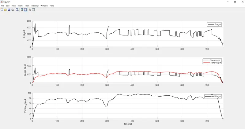
Fig 2

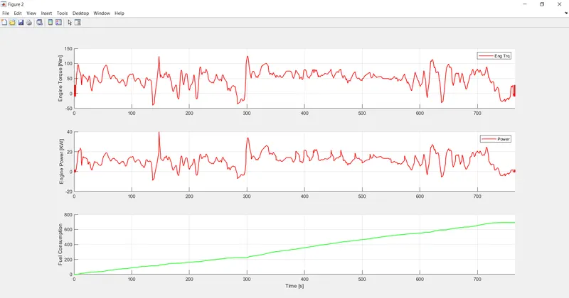
Fig 3

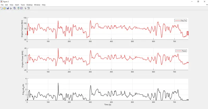
Fig 4

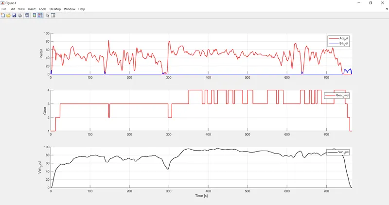
Fig 5

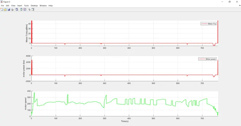
Fig 6

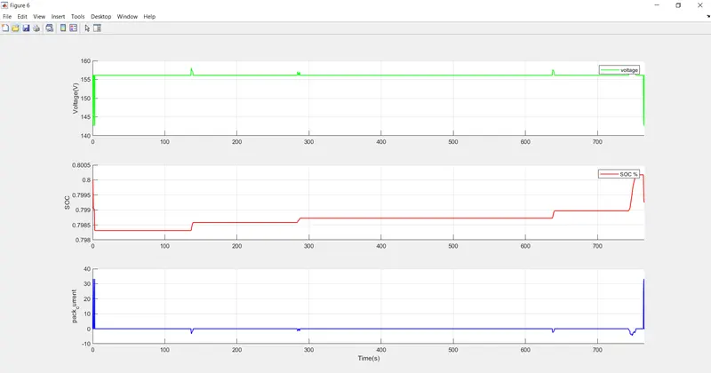
Fig 7

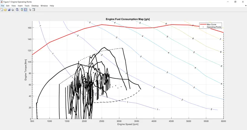
Fig 8

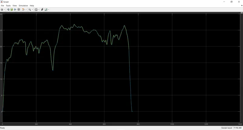
Fuel Economy of HWFET = 17.1706 (kmpl)

End:

The different exhibition qualities and working marks of UDDS and HWFET cycles are examined and the diagrams are plotted for

Motor, transmission input, transmission result and wheel speed wrt the time
Motor force, motor power, fuel rate and fuel utilization wrt the time
Gas pedal and brake pedal, gear order, vehicle speed, vehicle distance wrt the time
The motor working focuses on the motor fuel map
Engine speed, force, engine input power wrt the time
Pack voltage, current and SoC wrt the time
The engine working focuses on the engine input power map
Additionally, the efficiency numbers are arranged and contrasted and the venture 1