Project 2

DEVELOPMENT OF A FORWARD ENERGY BASED FUEL CONSUMPTION MODEL OF

P1 HYBRID VEHICLE

AIM:

To develop a forward energy-based fuel consumption model of a P1 hybrid vehicle by the modeling process, writing scripts in Matlab, modeling in Simulink and by analyzing data.

OBJECTIVE:

• To develop a forward energy-based fuel consumption model of a P1 hybrid vehicle by using writing scripts in Matlab, modeling in Simulink and by analyzing data.
• To simulate the vehicle on different drive cycles like UDDS, HWFET, FTP, NEDC,US06,WLDP using matlab scripts.
• To compute the fuel economy numbers for the P1 hybrid vehicle (kmpl) on the urban cycle (UDDS) and highway cycle (HWFET).
• To analyze the vehicle operating points in terms of engine speed, torque, transmission speeds, pedal positions, gear, distance travelled.
• To Plot the time trace for engine, transmission input, transmission output and wheel speed on one plot.
• To Plot engine torque, engine power, fuel rate and fuel consumption using subplots.
• To Plot accelerator and brake pedal, gear command, vehicle desired and actual speed, vehicle distance using subplots.
• To Plot the engine operating points on the engine fuel map.
• To Plot motor speed, torque, motor input power using subplots.
• To Plot pack voltage, current and SoC using subplots.
• To Plot the motor operating points on the motor input power map, with the motor max motoring and generating torque curves.
• To describing the vehicle behavior throughout the drive cycle and to generate the plots for both UDDS and HWFET cycle's.

INTRODUCTION:

HYBRID ELECTRIC VEHICLE (HEV):

A Hybrid Electric Vehicle (HEV) is a vehicle which is using two energy sources for propulsion of vehicle one energy source is storage, and the other is conversion of a fuel to energy, at least one of the energy sources being electrical energy by means of batteries (or) Mechanical energy by means of ultra flywheel/ultra capacitores (or) Hydrogen by means of fuelcells. The vast majority of hybrid electric vehicles are using a combination of petrol engines and electric motor.

FORWARD MODEL:

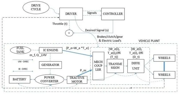
Forward models represent dynamic models with the correct causality. A forward-facing vehicle model features a driver model, which provides torque demand in the form of desired ICE & EM torque and brake torque (positive and negative torque), to meet the speed trace from a drive cycle.

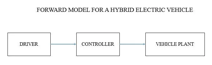
A basic driver model typically uses one or more Proportional-Integral (PI) controllers to achieve the torque demand, with reference to the desired speed trace. The torque produced by the ICE and EM propagates through the transmission and final drive ratios, before ending up as torque applied at the wheels. This is then exerted to the vehicle mass to force on the tire contact patch. The vehicle speed that results from applied force is propagated back through the drivetrain, and returns to the ICE and EM as angular velocity at the crankshaft. Brake torque applied directly at the wheels.

ELEMENTS OF HYBRID ELECTRIC VEHICLE FORWARD MODEL:

P1 HYBRID ARCHITECTURE:

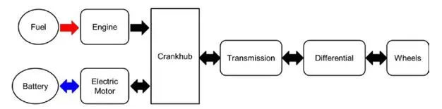
The P1 architecture, with the electric machine connected directly to the crankshaft. The electric motor functions as a generator, during vehicle deceleration, as an engine starter, and as a motor (to assist the engine) during vehicle accelerations.

DATA'S FOR ELECTRIC MOTOR & BATTERY:

Honda Insight motor and battery are considered for this project.

MATLAB SCRIPT:

INITIALIZATION FILE:

A Matlab script is used to load all the variables required for running the Simulink vehicle model and for post-processing data analysis.

%% Project 2 - HYBRID VECHILE MODELLING M-SCRIPT
% Initialization file for loading the variables for the hybrid vehicle simulation model
%% Vehicle Parameters
M = 1500;       % Vehicle weight [kg]
Cr = 0.015;     % Rolling resistance coefficient
Rw = 0.35;      % Rolling radius [m]
Cd = 0.33;      % Drag coefficient
Af = 2;         % Frontal area [m2]
rhoa = 1.225;   % Air density [kg/m3]
Vwind = 0;      % Wind velocity [kmph]
g = 9.81;       % Gravitational acceleration [m/s2]
theta = 0;      % Slope [deg]
myu_road_tire = 1; % Coefficient of friction between tire - road interface

%% Powertrain Parameters 
FDR = 3.73;                         % Final Drive Ratio / Diff Ratio
DiffEff = 0.99;                     % Differential efficiency (assumed independent of operating conditions)
NumGear = 4;                        % Number of gears in transmission
TransGear = (1:NumGear);            % Transmission Gears
TransRatio = [3.06, 1.62, 1, 0.7];  % Corresponding Transmission ratios
TransEff = 0.90;                    % Transmission efficiency (assumed independent of operating conditions)

TC_SR = [0, .5, .6, .7, .8, .87, .92, .94, .96, .97, 1];   % Torque Converter Speed Ratio (Matlab default) -> TurbSpd/PumpSpd  
TC_TR = [2.232, 1.5462, 1.4058, 1.2746, 1.1528, 1.0732, 1.0192, 1, 1, 1, 1];   % Torque Converter Torque Ratio (Matlab default) -> TurbTrq/PumpTrq
TC_Cf = 1e-4 * [.72558, .66322, .63463, .59042, .51331, .4144, .29287, .22444, .12186, .04386, 0]; % Torque Converter Capacity Factor (Matlab default) -> PumpTrq/PumpSpd^2 [Nm/rpm^2]

load Vehicle_Data/Engine_data_1_9L_Saturn_95kW
load Vehicle_Data/Trans_Shift_map
load Vehicle_Data/EM_Honda_Insight_10kW
load Vehicle_Data/ESS_NiMH6

%% BATTERY STATES

ESS_init_soc = 0.8;
ESS_soc_max = 0.9;
ESS_soc_min = 0.6;


%% Driver Parameters
Kp = 10;                    % P gain for driver PI model
Ki = 1;                     % I gain for driver PI model

%% Drive cycle values in m/s
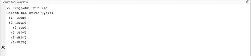
Drive_Cycle_Select = input(('Select the Drive Cycle:\n (1 -UDDS):\n (2-HWFET):\n   (3-FTP):\n  (4-US06):\n  (5-NEDC):\n  (6-WLTP):\n'));     % Drive cycle selection

if Drive_Cycle_Select == 1
    load DriveCycles/UDDS;
    
elseif Drive_Cycle_Select == 2
    load DriveCycles/HWFET;
    
elseif Drive_Cycle_Select == 3
    load DriveCycles/FTP;
    
elseif Drive_Cycle_Select == 4

    load DriveCycles/US06;
    
elseif Drive_Cycle_Select == 5
    load DriveCycles/NEDC;
    
elseif Drive_Cycle_Select == 6
    load DriveCycles/WLTP;
 
end

time_end = cyc_time(end);
vel_end = cyc_vel(end);

SELECTION OF DRIVE CYCLE:

• The drive cycle selection is done based on the user drive cycle input. The code as modified to select the drive cycle from the user inputs. By the user input, required drive cycle varibles are loded and simulink model is driven.

BLOCKS USED IN MODELLING:

• Goto - The Goto block passes its input to its corresponding From blocks. The input can be a real- or complex-valued signal or vector of any data type. From and Goto blocks allow you to pass a signal from one block to another without actually connecting them.
• From - The From block accepts a signal from a corresponding Goto block, then passes it as output. The data type of the output is the same as that of the input from the Goto block. From and Goto blocks allow you to pass a signal from one block to another without actually connecting them.
• Connection Port - The Connection Port block transfers a physical connection or signal across subsystem boundaries.
• Inport blocks - Inport blocks link signals from outside a system into the system.
• Outport blocks - Outport blocks link signals from a system to a destination outside of the system. they can connect signals flowing from a subsystem to other parts of the model. They can also supply external outputs at the top level of a model hierarchy.
• Constant block - The Constant block generates a real or complex constant value signal. This block to provide a constant signal input.
• PS Lookup Table (1D) - The PS Lookup Table (1D) block computes an approximation to function for a given data vectors. Both the input and the output are physical signals. The block generates output based on the input values using the selected interpolation and extrapolation methods.
• Scope - Scope block display time domain signals, the scope displays simulation results for attached input signals.
• Integrator - The Integrator block outputs the value of the integral of its input signal with respect to time.
• Gain - The Gain block multiplies the input by a constant value (gain). The input and the gain can each be a scalar, vector, or matrix. The input and gain are then multiplied, and the result is converted to the output data type using the specified rounding and overflow modes.
• STOP - Stops the simulation of the model.
• Saturation - The Saturation block produces an output signal that is the value of the input signal bounded to the upper and lower saturation values. The upper and lower limits are specified by the parameters Upper limit and Lower limit.
• Dynamic Saturation - The Saturation Dynamic block produces an output signal that is the value of the input signal bounded to the saturation values from the input ports up and lo.
• Rate Limiter - The Rate Limiter block limits the first derivative of the signal passing through it. The output changes no faster than the specified limit. The derivative is calculated using this equation:
• To work space - The to workspace block transfers the data to the workspace of matlab.
• Bus Creator - The Bus Creator block combines a set of input elements into a bus.
• Bus Selector - The Bus Selector block outputs the elements select from the input bus. The block can output the selected elements separately or in a new virtual bus. The Bus Selector block does not support mixing message and signal elements as outputs.
• Charts - A finite state machine is a representation of an event-driven (reactive) system. In an event-driven system, the system responds to an event by making a transition from one state (mode) to another. This transition occurs if the condition defining the change is true.
• Switch - The Switch block passes through the first input or the third input signal based on the value of the second input. The first and third inputs are data input. The second input is a control input. Specify the condition under which the block passes the first input by using the Criteria for passing first input and Threshold parameters.
• Sin - Sine of argument in radians
• Cos - Cosine of argument in radians
• Clock - The Clock block outputs the current simulation time at each simulation step. This block is useful for other blocks that need the simulation time.

FORWARD SIMULINK MODEL FOR P1 HYBRID VEHICLE:

SOLVER CONFIGURATION SELECTION:

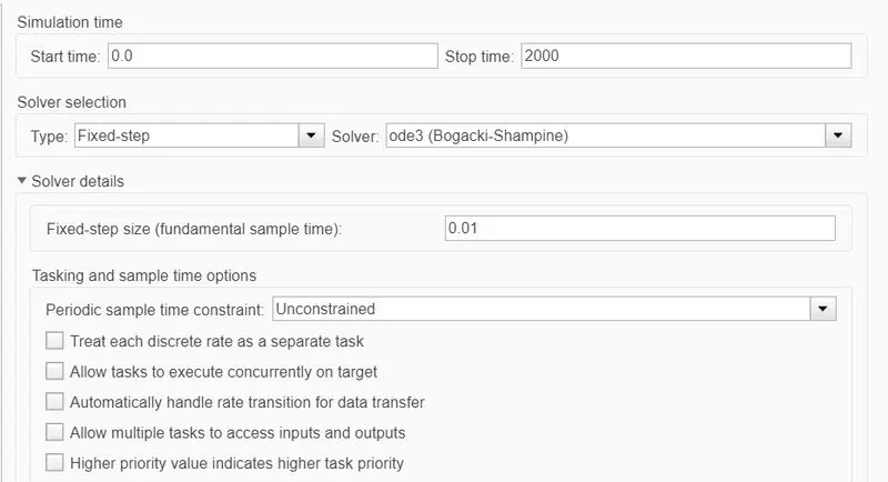
A solver computes a dynamic system's states at successive time steps over a specified time span. The solver selected is ode3 with a fixed step size of 0.01 sec.

DRIVER MODEL:

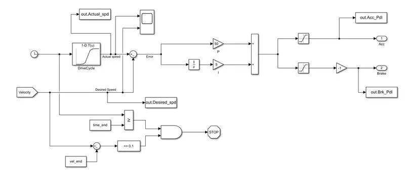
• The ‘Driver’ block, which is a basic PI controller that generates accelerator and brake pedal outputs to match the desired and actual vehicle speeds.
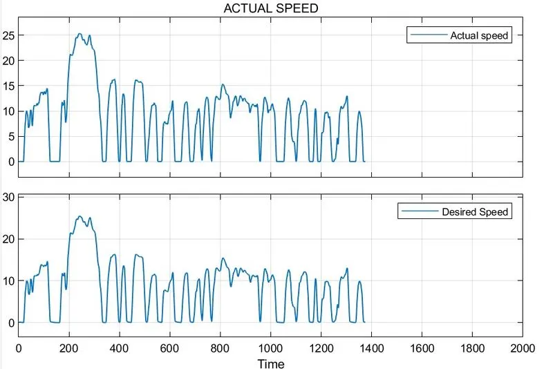
• The driver block uses the Drive cycle, A drive cycle is typically represented by a series of data points which plots vehicle speed against time. Driving cycles are produced to assess the performance of vehicles in various ways, including fuel consumption and pollutant emissions.
• The vehicle desired speed is provided in the relational operator and boolen condition based upon the simulation stop will execute.
• The saturation block limits the upper and lower conditions based on the limits provided.

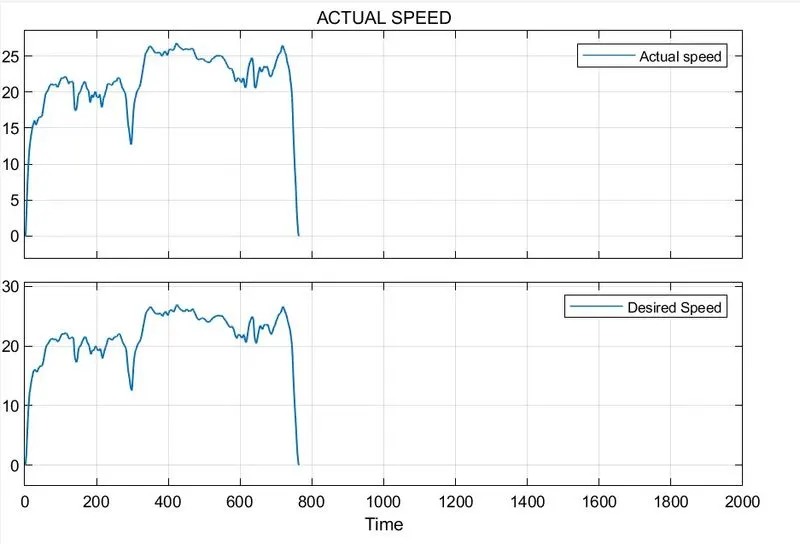
ACTUAL & DESIRED SPEED OF VEHICLE:

1. UDDS:

2. HWFET:

CONTROLLER MODEL:

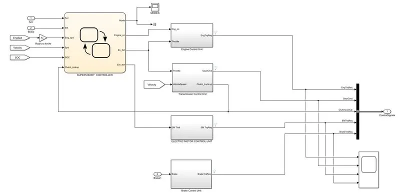
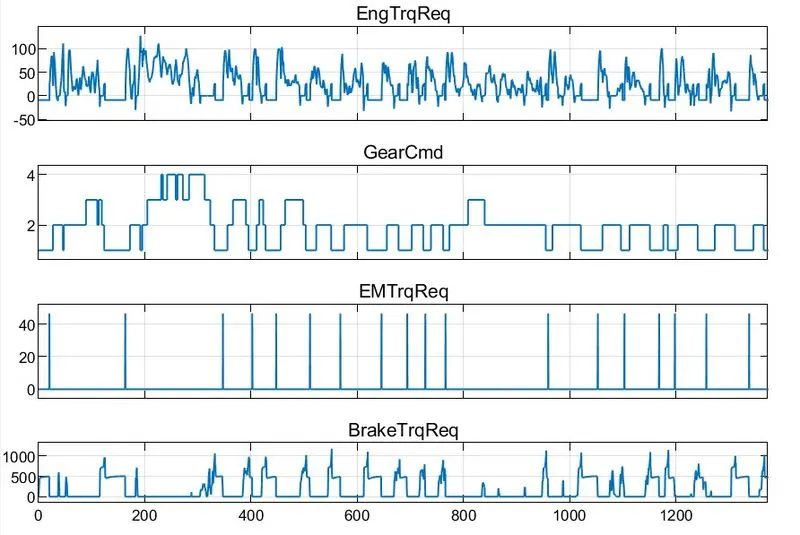
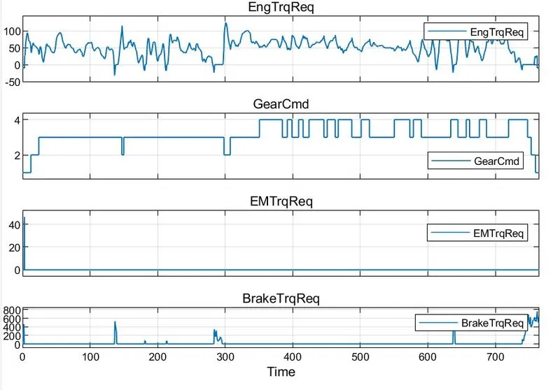
• The ‘Controller’ block is the brains of the vehicle, representing the electronic controls units which is deciced by the supervisory controller. Based on the driver inputs, it generates desired engine torque, desired electric motor controls, desired transmission shifting gear and desired brak torque.

SUPERVISORY CONTROLLER:

Supervisory control is a general term for control of many individual controllers or control loops, within a distributed control system. It refers to a high level of overall monitoring of individual process controllers, which is not necessary for the operation of each controller, but gives the operator an overall plant process view, and allows integration of operation between controllers.

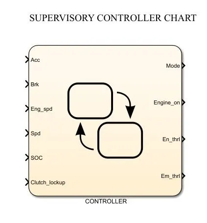
• The supervisory control chart shows the overall control system of the Vehicle system.
• From the driver inputs the Accelaration and braking inputs are assigned into the contol logic based on the user operated at the accelaration and applied braking the controls are controlled respectively.
• The engien speed are based on the engine operating conditions and also the SOC is based on the battery parameters are inputted into the contol logic system.
• based on the inputs by the user the control systems controls the statea at different operating conditions.
• This supervisory controller is for the hybrid electric vehicle to control the signals for internal combistion engine and also electric motor.

STATE FLOW CHART:

LOGIC EXPLANATIONS:

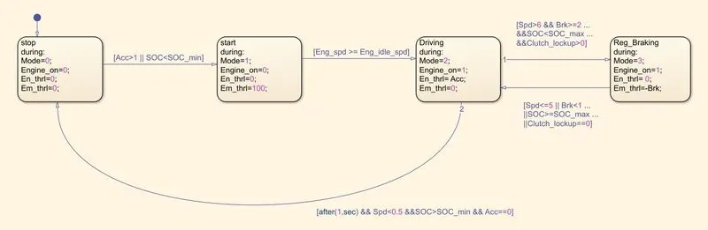
• The Supervisory control system consists of the four states,

(1). STOP

(2). START

(3). DRIVING

(4). REGENERATIVE BRAKING

(1). STOP:

• Based on the user inputs the signals are inoutted into the initial state of transition.
• In the stop state the mode is '0' at which the veicle is in static conditon.
• Also during the state the Engine and electric motor operating conditions are in 0 state.
• If the accelaration is provided by the user the transition takes place.

Transition From Mode-0 to Mode-1:- The transition of the state stop to start occurs when the accelaration is grater than 0 or the SOC is less than the Minimum SOC. if the condition statisfies the Modes are changed from stop to start.

(2). START:

• When the accelaration or SOC condition statisfies the start state enabled.
• In the start state the Mode is '1' @ start condition. For during the state the initial electric motor throttle will be 100.
• In start state the engine and engine throttle will be 0 state.

Transition From Mode-1 to Mode-2:- The transition of the state, start to Driving occurs when the Engine speed is grater than the Engine idle speed. if the condition statisfies the Modes are changed from start to Driving.

(3). DRIVING:

• In the driving state the engine speed will be grater then the engine idle speed. Therfore during the state the engine wil be '1' on state and engine throttle will be based on the accelaration inputted by the driver condition.
• In this state the electric motor throttle will be in off state '0'. The state will operated by using internal combustion engine.
• For the driving state Mode is '2'

Transition From Mode-2 to Mode-3:- The transition of the state, Driving to braking occurs when the Engine speed is grater than 6. The speed is based on the driver logic controller and Braking is grater than 2. Also, the SOC is lesser than maximum SOC and clutch lockup is grater than zero. if the condition statisfies the Modes are changed from Driving to braking.

(4). REGENRATIVE BRAKING:

• In hybrid electric vehicle the braking occurs when the transition conditions are statisfied and also Mode is '3'.
• During braking the motor act as a generator by this kinetic energy is converted into electrical energy by means of generator and the energies are stored in batteries.
• During the state ie: in Mode 4, the Engien state will be on '1' and electric motor throttle will be '-Brk' regenerative braking condition.

Transition From Mode-3 to Mode-1:- The transition of the state, Braking to stop occurs when the Engine speed is lesser than or equal to 5. The speed is based on the driver (input) logic controller or Braking is lesser than 1. Also, the SOC is grater than maximum SOC or clutch lockup is equal to zero. if the condition statisfies the Modes are changed from Braking to stop after 1 second.

• The state logic controlles the logics of stop, start, driving and braking conditions based on the user inputs and also the transition occurs if the conditions are statisfied.

INPUT & OUTPUT PANE:

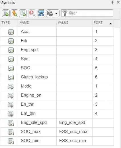
The Symbols pane are used to:

ENGINE CONTROL UNIT:

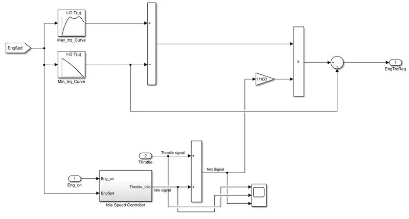
• The Engine control unit derives the Engine speed to execute the Engine torque requirement.
• In the Engine contol unit the maximum and minimum torqure are mapped using 1-D look up table and the signals are combained with the idele speed controller.

IDLE SPEED CONTROLLER:

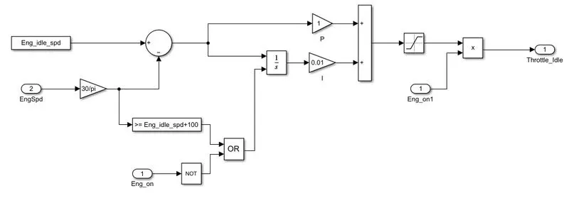
• In the Engine control unit block the Engine idle speed is saturated to execute the Trottle idle speed.
• In which the Engine speed is gained and integrated using integrator block with respect to the time.
  
• Also, the engine ON is provided to execute when the control unit driving state is accuated.
• The logical operaters are used to decide the control of engine on when it is in idle speed or NOT.

TRANSMISSION CONTROL UNIT:

• In the transmission control unit Throttle and vehicle speed are inputted into the gear transmission logic control system.
• Based upon the vehicle speed and throttle reponse the gear command are controlled.

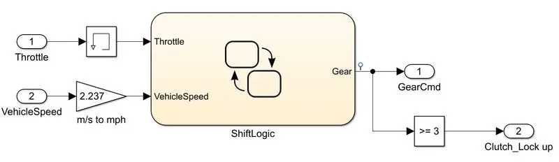
• In the transmission control unit the clutch lock up is provided to engage and disengage when the vehicle speed is at maximum range.

GEAR SHIFT LOGIC:

• Based on the Vehicle speed and throttle response the gears are selected based on the state and during conditions.

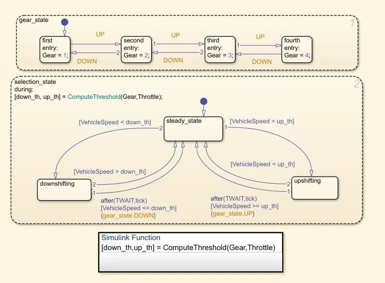
• The up and down gears are shifted based upon the conditions and actions on the logics.
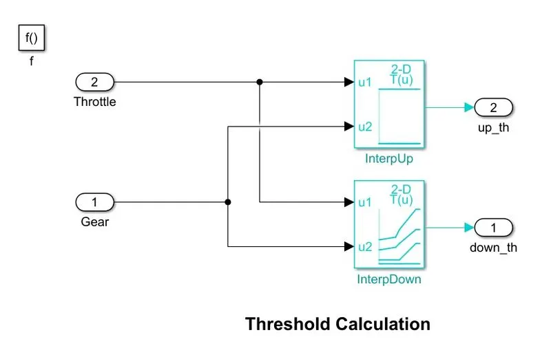
• Based on the simulink function using 2-D look up table to mapp the up shifting and down shifting conditions.

ELECTRIC MOTOR CONTROL UNIT:

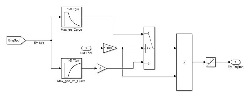
• The Electric motor control unit derives the Electric motor speed to execute the motor torque requirement.
• In the Electric motor control unit the maximum and minimum torqure are mapped using 1-D look up table and the signals are decicded based on the switch block inputs condition with motor trottle.

BRAKE CONTROL UNIT:

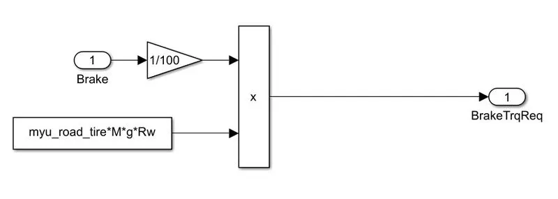
• The brake control unit is contolled based on the mass, gravity, wheel radius and the co-efficient of friction between the tire and the road surfaces.
• The brake and the Tire load's are multipled to execute the brake torqur requirements.

CONROL SIGNALS:

1. UDDS:

2. HWFET:

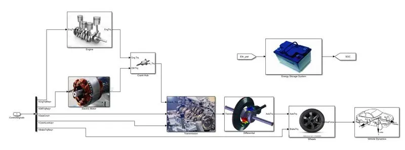
POWERTRAINS MODEL:

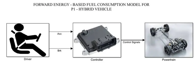
• The ‘Powertrain’ block which represents the drivetrain of the vehicle. It consists of an ‘Engine’ connected to the ‘Automatic Transmission’ through a ‘Torque Converter’. The output of the transmission is connected to the ’Differential’, which powers the ‘Wheels’, that provides the tractive force for vehicle acceleration. The longitudinal dynamics of the vehicle along with the road load is represented in the ‘Vehicle Dynamics’ block.

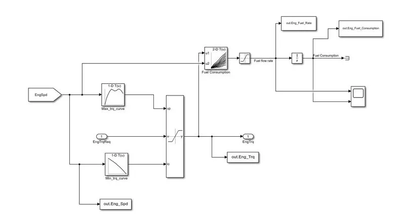
ENGINE MODEL:

• The Engine model is modelled using the Engine speed and Engine torque requirement.
• Based on the Engine torque and Engine speed the maximum and minimum torque are mapped using 1-D look up table and that are saturated using upper and lower limits.
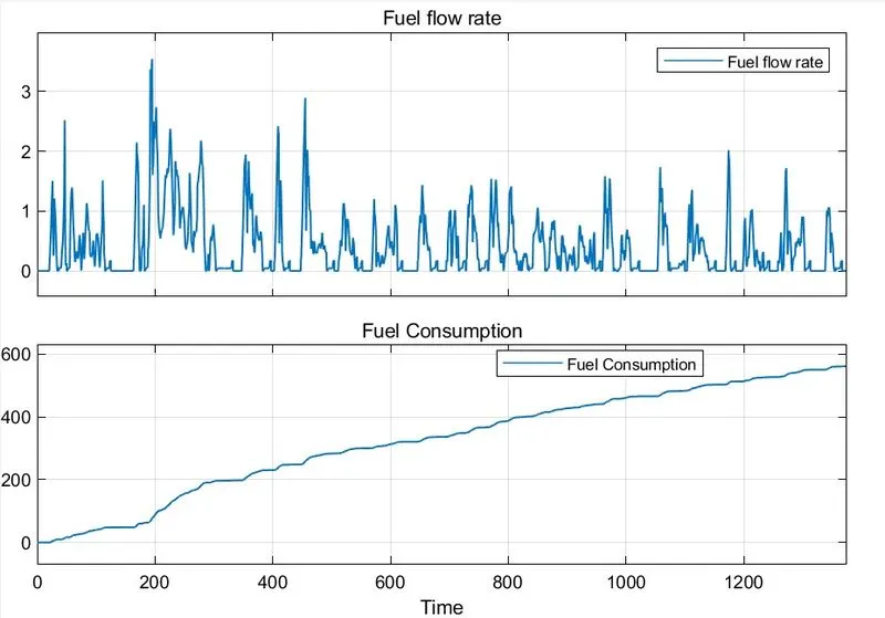
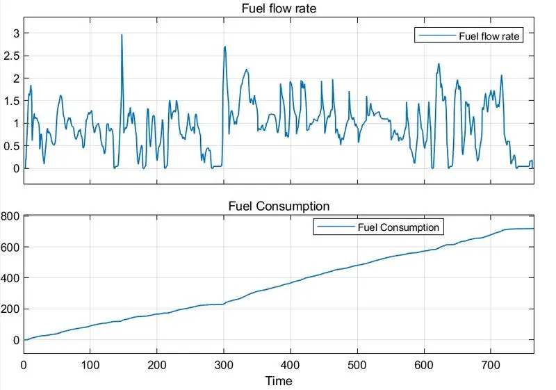
• The saturated executes the Engine fule rate and the integration of fuel flow rate gives the Fuel consumption of the engine.

ENGINE FUEL CONSUMPTION AND FLOW RATE:

1. UDDS:

2. HWFET:

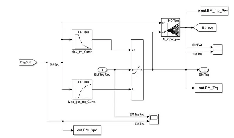
ELECTRIC MOTOR MODEL:

• The Electric Motor model is modelled using the Motor speed and Motor torque requirement.
• Based on the Electric motor torque and Electric motor speed the maximum and minimum torque are mapped using 1-D look up table and that are dynamically saturated using upper and lower limits.
• The saturated executes the Electric power whic are mapped using 2-D look up table.
• The Electric power are used in determining the battery perfomance.

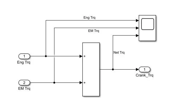
CRANK HUB MODEL:

• In the crank hub the Engine and Electric Motor torques are combined to make the crank torque.
• The modelling was based on te P1 Hybrid architecture.
• In which the Electric Motor are connected with the crank of the engine and combined togeter to get the crank torque whic are inputted into the transmission unit.

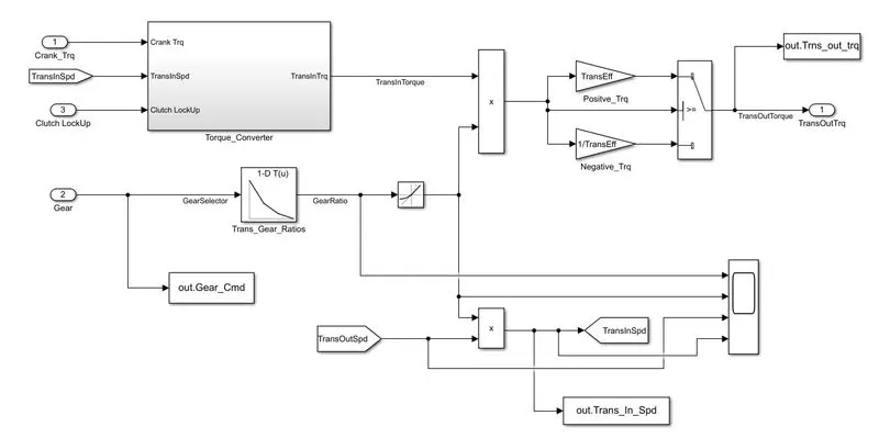
TRANSMISSION MODEL:

• The crank torque, Clutch lockup and the Gear transmission are inputted into the transmission block.
• Based upon the transmission input torque and transmission output speed the positive and negative efficiencies are determined using switch thershold conditions.
• From which the transmission output torque's are derived.

TORQUE CONVERTER:

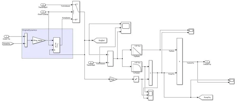
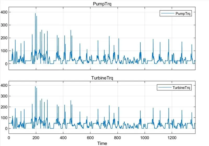
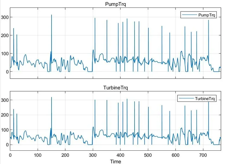
• In the torque conveter the pump and turbine Torque's are determined by using the 1-D mapped models.
• The pump torque are derived by using the C- factor mapped 1-D model.
• The clutch lockup is provided, based upon the supervisory controller command the clutch lockup is activated to engage and disengage in the torque converter at certain speed range.
• In whic the clutch lockup is engaged to transmit the engine speed to integrated with respect to the simulation time.

PUMP AND TURBINE TORQUE:

1. UDDS:

2. HWFET:

ENERGY STORAGE SYSTEM MODELLING:

Zeroth Order Equivalent circuit model:

The battery can be modeled by means of a zero-th order equivalent circuit, where the cell open circuit voltage (v_oc), is in series with an equivalent resistance, (R) . Both these parameters are functions of battery state of charge (SoC).

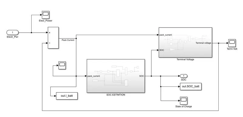
• From the inport block the Electric power from the electric motor unit are extracted and inputted into the energy storage system.
• Based on the time the current Amps are plotted.
• Forming a loop from the terminal voltage connected to the pack_current as a closed loop.
• In that the SOC and terminal voltage are to be determined.

SOC ESTIMATION:

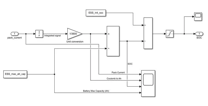
• For the estimation of SOC the pack_current array's are integrated and conveterd from coloumb to A/hr by dividing it into 3600.
• Then, the Battery maximum ah capacity is divided with that pack_current to determine the SOC of the battery pack_data.
• Also. by considering the initial state of charge as 100% (0.8), to subtract with the determined SOC and saturated by using saturation block.
• The upper and lower limits are assigned as 0 and 1.

TERMINAL VOLTAGE ESTIMATION:

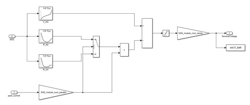
• By the determination of SOC, the terminal voltage are detremined by using the estimated SOC and provided Pack_current data,
• The pack_current are connected with the gain block to estimate the number of cells connected in parallel.
• The determined SOC are inputted to estimate the pack_current terminal voltages.
• The internal resistance (Discharge & charge) are mapped using 1-D look up table as a function of ESS_data SOC.
• Also, the V_oc are mapped using 1-D look up table with an input of determined SOC and as a function of ESS_data SOC.
• By model's are derived by the equation of zeroth order equivalent circuit and saturated using saturation block.
• In the saturation block the Maximum limits are assigned as Max_volts (9) and lower limits are assigned as Min_volts as (6).
• Basd on the saturated voltage are multiplied with number of cells connected in series by which the terminal voltage are been determined.

DIFFERENTIAL MODEL:

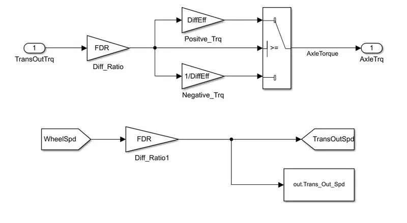
• The transmission output torque is inputted into the gain of Final Drive Ratio (FDR), by which the positive and negative differential efficiencies are derived by using switch treshold conditions.
• From te the axle torque are determined.
• The wheel speed from the vehicle is inputted to compute the transmission output speed.

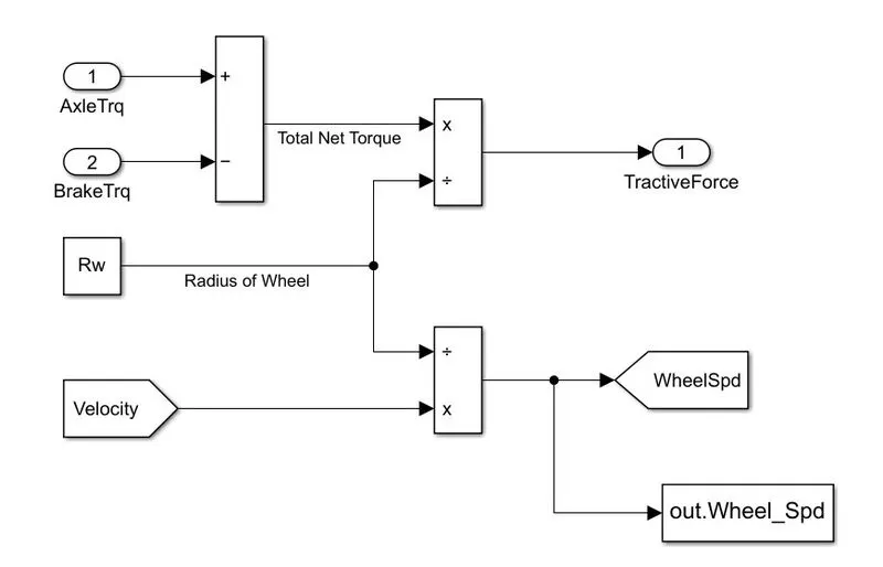
WHEEL MODEL:

• The net torque Axle torque and the Brake torque are transmitted into the wheel and the weel radius are determined to estimate the tractive forces.
• The wheel speed is determined by using the velocity of the vehicle and te wheel radius.

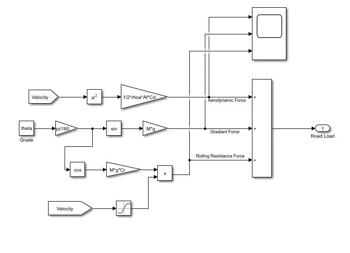
ROAD LOAD:

• The Road Load is a combination of all the forces acting on the vehicle.
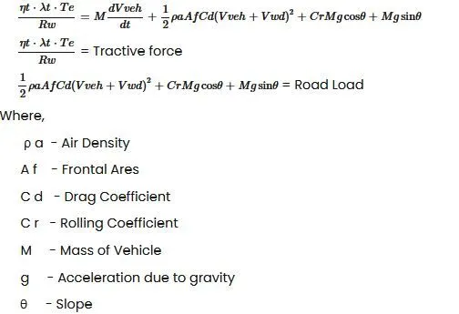
• The rolling resistance force, Gradient forces, Aerodynamic forces are the resultant of all the load's are called as road load.

• From the road load the Tractive force is calculated as,

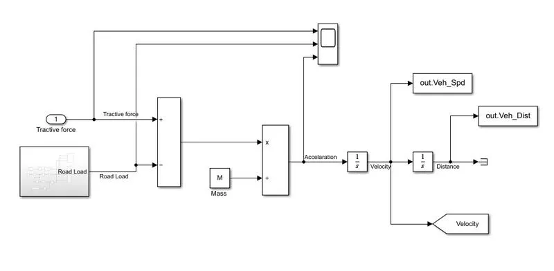
VEHICLE DYNAMICS:

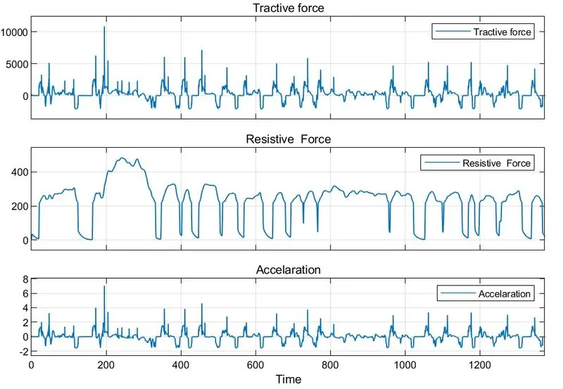
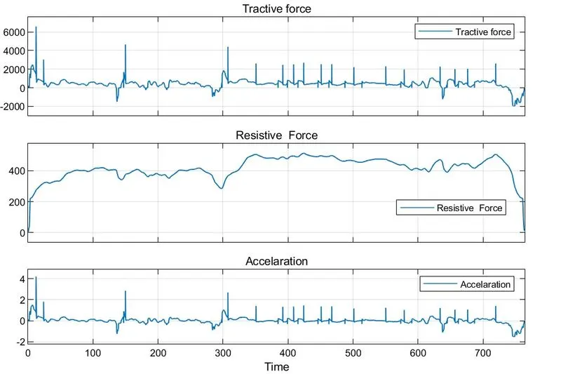
• The vehicle dynamics is the motion of the vehicle generated by the steering action, through which the vehicle is capable of independent motion. In a vehicle several forces act on it and the net or resultant force governs the motion according to the Newton's second law. The propulsion unit of the vehicle delivers the force necessary to move the vehicle forward. This force of the propulsion unit helps the vehicle to overcome the resisting forces due to gravity, air and tire resistance.

DYNAMIC FORCES AND LOAD'S:

1. UDDS:

2. HWFET:

MATLAB SCRIPT:

POST PROCESSING FILE:

The post processing file script is used to analyze data and to generate the plots.

%% Post-Processing File
% Project 2 - P1 Hybrid Electric Vehicle Model
% Simulink results for post-processing of the data analysis.
close all
%% Assigning variables
Time = out.tout;
Acc_Pdl = out.Acc_Pdl;                  % Accelerator pedal [%]
Brk_Pdl = out.Brk_Pdl;                  % Brake pedal [%]
Gear_Cmd = out.Gear_Cmd;                % Transmission gear
Trans_In_Spd = out.Trans_In_Spd*30/pi;  % Transmission input speed [rpm]
Trans_Out_Spd = out.Trans_Out_Spd*30/pi;% Transmission output speed [rpm]
Eng_Trq = out.Eng_Trq;                  % Engine brake torque [Nm]
Eng_Spd = out.Eng_Spd*30/pi;            % Engine speed [rpm]
Eng_fuel_rate=out.Eng_Fuel_Rate;        % Engine fuel rate
Eng_Fuel_Consump = out.Eng_Fuel_Consumption;    % Engine fuel consumption [g]
Veh_Dist = out.Veh_Dist/1000;           % Distance traveled by vehicle [km]
Veh_Spd = out.Veh_Spd*18/5;             % Vehicle speed [kmph]
Desired_Spd=out.Desired_spd*18/5;       % Desired speed (Kmph)
Wheel_Spd=out.Wheel_Spd*30/pi;          % Wheel speed (rpm)
EM_Spd=out.EM_Spd;
EM_Trq=out.EM_Trq;
EM_Inp_Pwr=out.EM_Inp_Pwr;
V_batt=out.V_batt;
I_batt=out.I_batt;
SOC_batt=out.SOC_batt;

%% Data Analysis
Eng_Pwr = Eng_Spd*pi/30*Eng_Trq/1000;   % Engine brake power [kW]
rho_petrol = 0.7197;                    % Density of petrol [kg/L]
Veh_Distance=(out.Veh_Dist.Data(:,1))/1000;
Eng_Fuel_Consumption = out.Eng_Fuel_Consumption.Data(:,1); 
kmpl = Veh_Distance(end)/(Eng_Fuel_Consumption(end)/1000/rho_petrol);    % Fuel economy [kmpl] 

% Fuel Economy for Engine;
T=table({'FUEL ECONOMY'},(kmpl));
T.Properties.VariableNames={'ENGINE','KMPL'}
writetable(T,'UDDS.xlsx','Sheet',1);
%% PLOTTING
%% PLOTTING THE DRIVE CYCLE
figure(1)
plot(cyc_time,cyc_vel,'LineWidth',1,'Color','r')
grid on
xlabel('TIME (Sec)')
ylabel('VELOCITY (Mph)')
title('DRIVE CYCLE')
legend('Drive cycle')

%% 1 - Plotting for the time trace for engine
figure(2)
hold on
plot(Time,Trans_In_Spd,'linewidth',0.5,'color','r')
plot(Time,Trans_Out_Spd,'linewidth',0.5,'color','k')
plot(Wheel_Spd,'linewidth',0.5,'color','b')
grid on
xlabel('TIME (Sec)')
ylabel('SPEED (Rpm)')
legend('Trans In Spd','Trans Out Spd','Wheel Spd')
title('TIME TRACE FOR ENGINE')
subtitle('TRANS IN SPD -TRANS OUT SPD - WHEEL SPD')

%% 2. PLOTTING FOR ENGINE AND FUEL PARAMETERS
figure(3)
subplot(4,1,1)
plot(Eng_Trq)
xlabel('TIME (Sec)')
ylabel('TORQUE (Nm)')
legend('Torque')
title('ENGINE TORQUE')
grid on
subplot(4,1,2)
plot(Eng_Pwr)
xlabel('TIME (Sec)')
ylabel('POWER (Kw)')
legend('Power')
title('ENGINE POWER')
grid on
subplot(4,1,3)
plot(Eng_fuel_rate)
xlabel('TIME (Sec)')
ylabel('FUEL RATE')
legend('Fuel Rate')
title('ENGINE FUEL RATE')
grid on
subplot(4,1,4)
plot(Eng_Fuel_Consump)
xlabel('TIME (Sec)')
ylabel('FUEL CONSUMP (g)')
title('ENGINE FUEL CONSUMPTION')
legend('Fuel consumption')
grid on

%% PLOTTING FOR ACCELARATOR & BRAKE PEDAL, GRAR COMMANDS,VEHICLE SPEEDS, VEHICLE DISTANCE
figure(4)
subplot(4,1,1)
grid on
hold on
plot(Time,Acc_Pdl,'color','r')
plot(Time,Brk_Pdl,'color','g')
xlabel('TIME (Sec)')
ylabel('Pedal %')
title('ACC & BRK PEDAL')
legend('Acc','Brk')
subplot(4,1,2)
grid on
hold on
plot(Time,Gear_Cmd,'color','g')
xlabel('TIME (Sec)')
ylabel('Gear')
title('GEAR COMMAND')
legend('Gear')
subplot(4,1,3)
grid on
hold on
plot(Desired_Spd,'color','r')
plot(Veh_Spd,'color','g')
xlabel('TIME (Sec)')
ylabel('Speed (Kmph)')
title('DESIRED AND ACTUAL SPEED')
legend('Desid Spd','Act Spd')
subplot(4,1,4)
grid on
hold on
plot(Time,Veh_Distance)
xlabel('TIME (Sec)')
ylabel('Distance (Km)')
title('VEHICLE DISTANCE')
legend('Distance')


%% PLOTTING ENGINE OPERATING POINTS FOR ENGINE FUEL MAP
figure('Name','ENGINE OPERATING POINTS');
hold on
grid on
title('Engine Operating Points','fontsize',12);
p1=plot(Eng_map_spd*30/pi,Eng_max_trq,'linewidth',2,'color','r');
p2=line([Eng_map_spd(end)*30/pi Eng_map_spd(end)*30/pi],[0 Eng_max_trq(end)]);
set(p2,'linewidth',1,'linestyle','--','color','k');
p3=line([Eng_map_spd(1)*30/pi Eng_map_spd(1)*30/pi],[0 Eng_max_trq(1)]);
set(p3,'linewidth',1,'linestyle','--','color','k');
[c,h] = contour(Eng_map_spd'*30/pi,Eng_map_trq,Eng_fuel_map');
clabel(c,h);
xlabel('Engine Speed [rpm]');
ylabel('Engine Torque [Nm]');
title('Engine Fuel Consumption Map [g/s]');
legend([p1 p3],{'Torque Curve','Operating Points'},'Location','southwest');
axis([Eng_map_spd(1)*30/pi Eng_map_spd(end)*30/pi 0 Eng_map_trq(end)])

%% PLOTTING MOTOR SPEED , TORQUE AND MOTOR POWER
figure(6)
subplot(3,1,1)
plot(EM_Spd)
xlabel('TIME (Sec)')
ylabel('SPEED (Rpm)')
legend('Speed')
title('MOTOR SPEED')
grid on
subplot(3,1,2)
plot(EM_Trq)
xlabel('TIME (Sec)')
ylabel('TORQUE (Nm)')
legend('Torque')
title('MOTOR TORQUE')
grid on
subplot(3,1,3)
plot(EM_Inp_Pwr)
xlabel('TIME (Sec)')
ylabel('MOTOR POWER (W)')
legend('Input Power')
title('MOTOR POWER')
grid on

%% PLOTTING VOLTAGE, CURRENT AND SOC
figure(7)
subplot(3,1,1)
plot(V_batt)
xlabel('TIME (Sec)')
ylabel('VOLTAGE (V)')
legend('Battery Voltage')
title('BATTERY VOLTAGE')
grid on
subplot(3,1,2)
plot(I_batt)
xlabel('TIME (Sec)')
ylabel('CURRENT (A)')
legend('Battery Current')
title('BATTERY CURRENT')
grid on
subplot(3,1,3)
plot(SOC_batt)
xlabel('TIME (Sec)')
ylabel('STATE OF CHARGE (%)')
legend('SOC')
title('STATE OF CHARGE')
grid on

%% PLOTTING MOTOR OPERATING POINTS ON MOTOR INPUT POWER MAP
figure('Name','ELECTRIC MOTOR OPERATING POINTS');
hold on
grid on
title('Engine Operating Points','fontsize',12);
p1=plot(EM_map_spd*30/pi,EM_max_trq,'linewidth',2,'color','r');
p4=plot(EM_map_spd*30/pi,EM_max_gen_trq,'linewidth',2,'color','g');
p2=line([EM_map_spd(end)*30/pi EM_map_spd(end)*30/pi],[EM_max_gen_trq(end) EM_max_trq(end)]);
set(p2,'linewidth',1,'linestyle','--','color','k');
p3=line([EM_map_spd(1)*30/pi EM_map_spd(1)*30/pi],[EM_max_gen_trq(1) EM_max_trq(1)]);
set(p3,'linewidth',1,'linestyle','--','color','k');
[c,h] = contour(EM_map_spd'*30/pi,EM_map_trq,EM_inpwr_map');
clabel(c,h);
xlabel('Motor Speed [rpm]');
ylabel('Motor Torque [Nm]');
title('ELECTRIC MOTOR POWER MAP [W]');
legend([p1 p4 p3],{'Torque Curve','Regen Curve','Operating Points'});
axis([EM_map_spd(1)*30/pi EM_map_spd(end)*30/pi EM_max_gen_trq(1) EM_max_trq(1)])

ANALYSING DATA'S:

1. UDDS DRIVE CYCLE DATA ANALYSIS AND PLOTTINGS:

a. Tabulate the fuel economy numbers (kmpl) for UDDS cycle,

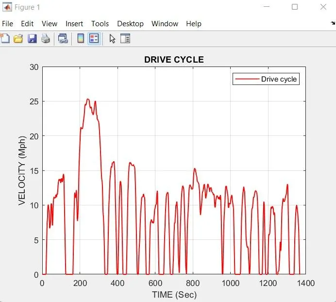
UDDS DRIVE CYCLE:

• A drive cycle is typically represented by a series of data points which plots vehicle speed against time. Driving cycles are produced to assess the performance of vehicles in various ways, including fuel consumption and pollutant emissions.

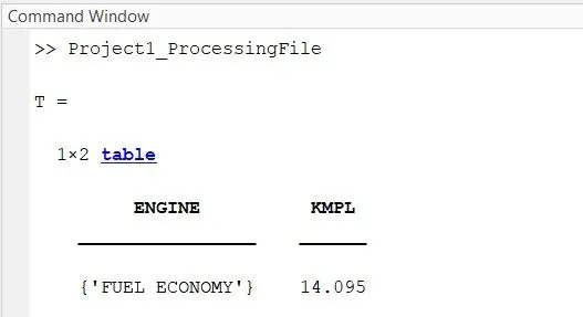
FUEL ECONOMY NUMBERS FOR UDDS CYCLE (CONVENTIONAL VEHICLE):

FUEL ECONOMY NUMBERS FOR UDDS CYCLE (P1 HYBRID VEHICLE):

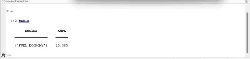
• From the UDDS drive cycle the computation as been done and for that 15.385 kmpl of fuel economy is obsorved.
• Compared to Conventional vehicle @ fuel economy 14.095 the P1 Hybrid vehicle fuel economy will be higher.

b. Plotting the time trace for engine, transmission input, transmission output and wheel speed on one plot:

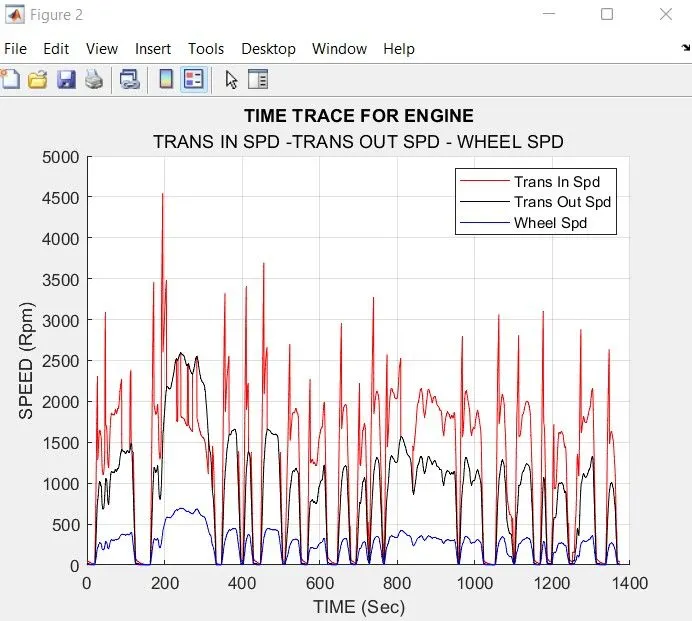
• The plot describes the time and the speed of an engine.
• In this, the transmission input speed, transmission output speed and the wheel speed are plotted.
• Depending on the Desired velocity of the vehicle the wheel speed is computed with wheel radius.
• From the wheel speed, the transmission ouput speed is computed based on the FDR in the differential unit.
• The Transmission input speed is evaluated by the transmission output speed , gear ratio's and the transmission inout torque.

c. Plotting for engine torque, engine power, fuel rate and fuel consumption using subplots:

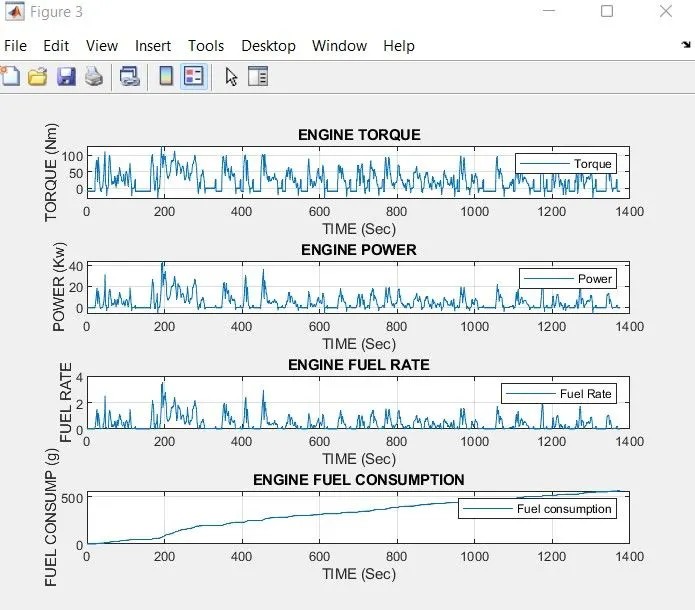
• The Engine torque is determined by the Dynamic saturation block, with this the maximum and minimm torque requirements are saturated based on upper and lower limits.
• The engine power is derived based on the engine speed and engine torque requirements.
• Based on the Engine torque and Engine speed the maximum and mnimum torque are mapped using 1-D look up table and that are saturated using upper and lower limits.
• The saturated executes the Engine fule rate and the integration of fuel flow rate gives the Fuel consumption of the engine.

d. Plotting the accelerator and brake pedal, gear command, vehicle desired and actual speed, vehicle distance using subplots:

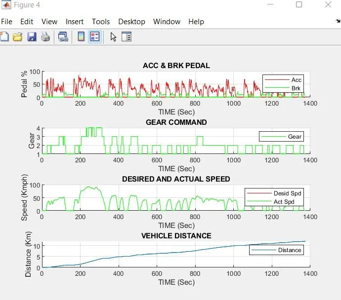
• The plot describes the Vehicle behaviour of the engine parameters and user inputs.
• From the desired and actual drive velocities the axle and brake pedals are specified by the driver inouts.
• Based on the inputs, in the transmission system the Gear ratio's are shifted based on the velocities and torque's.
• The disance of the vehicle is determined by the integration of the desired velocity by the vehicle.

e. Plotting the engine operating points on the engine fuel map:

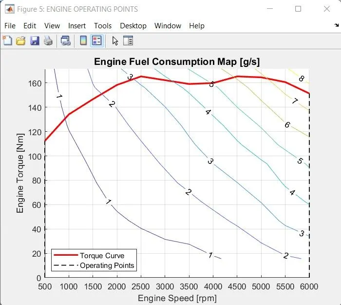
• The potting has been done for the maps with engine speed on x-axis and engine brake torque on y-axis, and the Engine operating points are represented using contour function.
• From the plotting, the engine maximum and minum torque's are identified and also the operating conditions are determined.
• The Engine fuel consumption is estimated by using the fuel map, based on the engine speed and engien torque @ operating conditions the fuel consumption of the vehicle is obtained.

f. Plotting the Electric Motor speed, Torque and Motor input power:

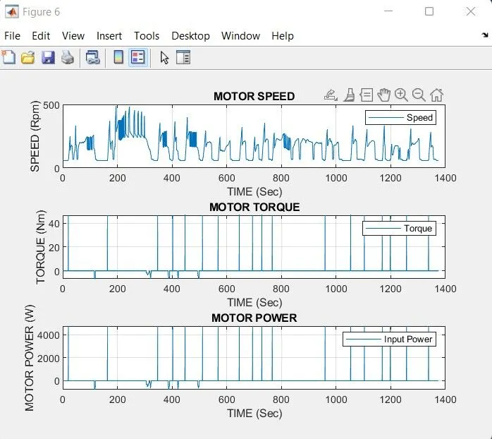
• The plot describes the Motor speed and Motor torque and motor power requirement.
• Based on the Electric motor torque and Electric motor speed the maximum and minimum torque are mapped using 1-D look up table and that are dynamically saturated using upper and lower limits from the Electric machine unit and by the electric motor control unit.
• The saturated executes the Electric power which are mapped using 2-D look up table from which the motor input power are mapped with respect to the electric motor speed and torque.
• The Electric power are used in determining the battery perfomance.

g.Plotting the Voltage, Current and State of charge using subplots:

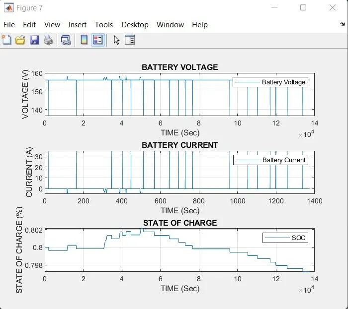
• Based on the time the Current (Amps), Voltage(V) and State of charge (SOC %) are varied accordingly.
• From the plotting it is obsorved that the initial state of charge would be 80% after the certain time intervel the state of charge will be varried according to the accelaration and delaration and regenerative braking commands by the control units as the discharging state..
• After that with constant time the SOC remains same as in the current are in constant state.
• Also. by considering the initial state of charge as 80% (0.8), to subtract with the determined SOC and saturated by using saturation block.
• The upper and lower limits are assigned as 0 and 1 of SOC during monetering and regenrative brakings.
• During charging, discharging and constant states the signals are varied respectively with same battery capacity as it connected in series.

h. Plotting the electric motor operating points on the motor input power map:

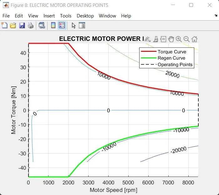
• The potting has been done for the maps with motor speed on x-axis and motor torque on y-axis, and the Electric motor points are represented using contour function.
• From the plotting, the motor monetering and generating torque's are identified and also the operating conditions are determined.
• The Regenerative braking is estimated by using the motor power map, based on the motor speed and motor torque @ operating conditions the power requirements of the vehicle is obtained.

2. HWFET DRIVE CYCLE DATA ANALYSIS AND PLOTTINGS:

a. Tabulate the fuel economy numbers (kmpl) for HWFET drive cycle:

HWFET DRIVE CYCLE:

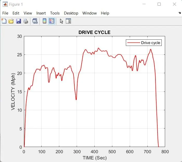
• A drive cycle is typically represented by a series of data points which plots vehicle speed against time. Driving cycles are produced to assess the performance of vehicles in various ways, including fuel consumption and pollutant emissions.

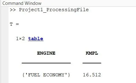
FUEL ECONOMY NUMBERS (CONVENTIONAL VEHICLE):

FUEL ECONOMY NUMBERS (P1 HYBRID VEHICLE):

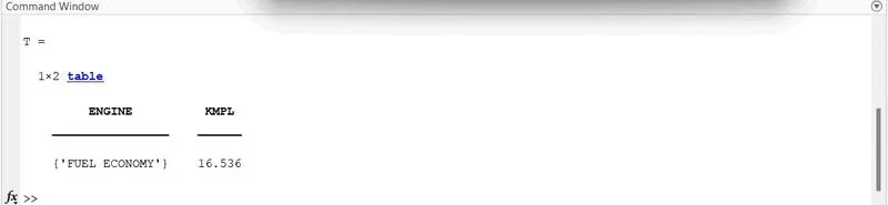
• From the HWFET drive cycle the computation as been done and for that 16.536 kmpl of fuel economy is obsorved.
• Compared to Conventional vehicle @ fuel economy 16.512 the P1 Hybrid vehicle fuel economy will be higher and much efficient in HWFET drive cycle.

b. Plotting the time trace for engine, transmission input, transmission output and wheel speed on one plot:

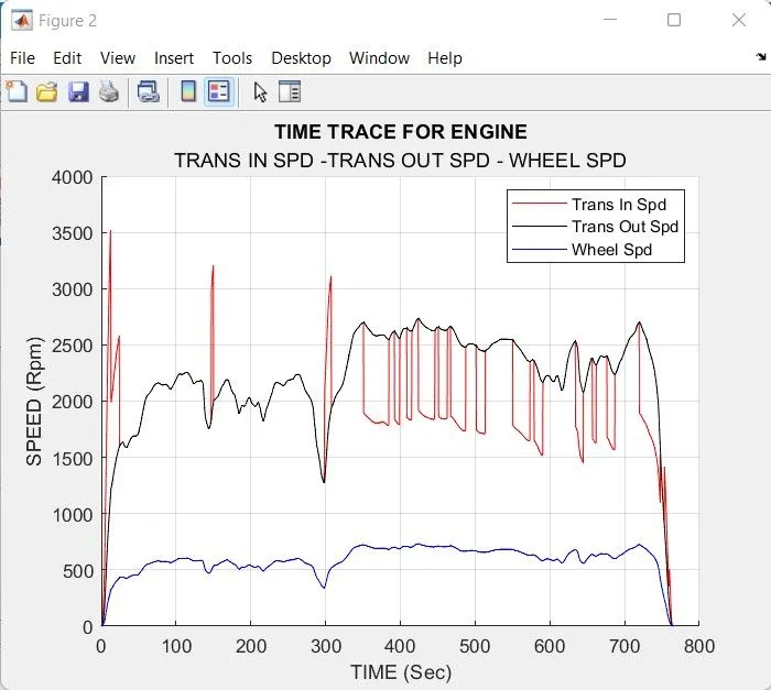
• The plot describes the time and the speed of an engine.
• In this, the transmission input speed, transmission output speed and the wheel speed are plotted.
• Depending on the Desired velocity of the vehicle the wheel speed is computed wit wheel radius.
• From the wheel speed, the transmission ouput speed is computed based on the FDR in the diffential unit.
• The Transmission input speed is evaluated by the transmission output speed , gear ratio's and the transmission inout torque.

c. Plotting the engine torque, engine power, fuel rate and fuel consumption using subplots:

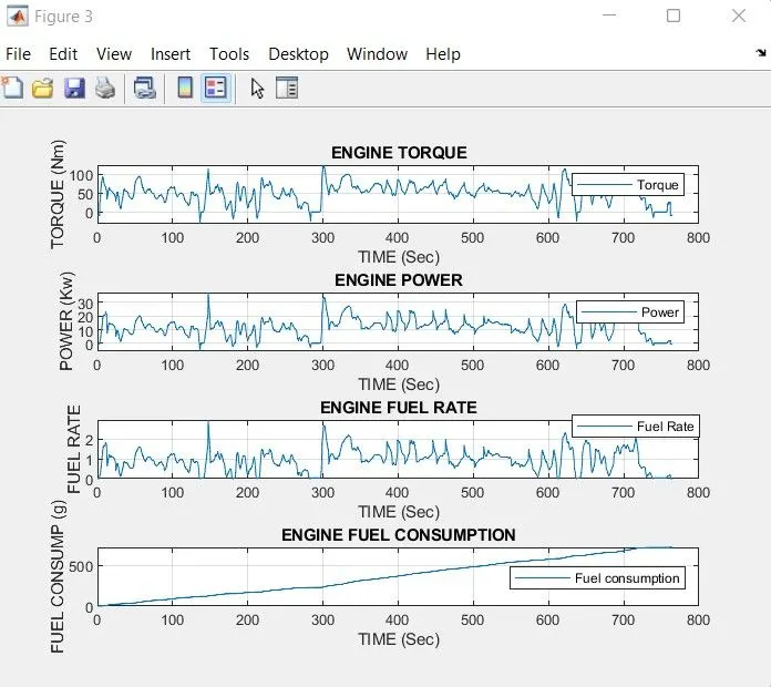
• The Engine torque is determined by the Dynamic saturation block, with this the maximum and minimm torque requirements are saturated based on upper and lower limits.
• The engine power is derived based on the engine speed and engine torque requirements.
• Based on the Engine torque and Engine speed the maximum and mnimum torque are mapped using 1-D look up table and that are saturated using upper and lower limits.
• The saturated executes the Engine fule rate and the integration of fuel flow rate gives the Fuel consumption of the engine.

d. Plotting the accelerator and brake pedal, gear command, vehicle desired and actual speed, vehicle distance using subplots:

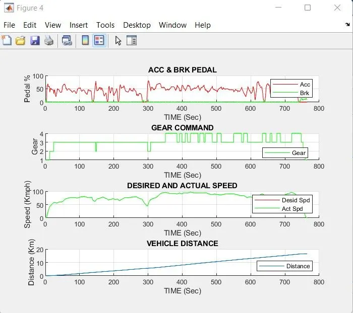
• The plot describes the Vehicle behaviour of the engine parameters and user inputs.
• From the desired and actual drive velocities the axle and brake pedals are specified by the driver inouts.
• Based on the inputs, in the transmission system the Gear ratio's are shifted based on the velocities and torque's.
• The disance of the vehicle is determined by the integration of the desired velocity by the vehicle.

e. Plotting the engine operating points on the engine fuel map:

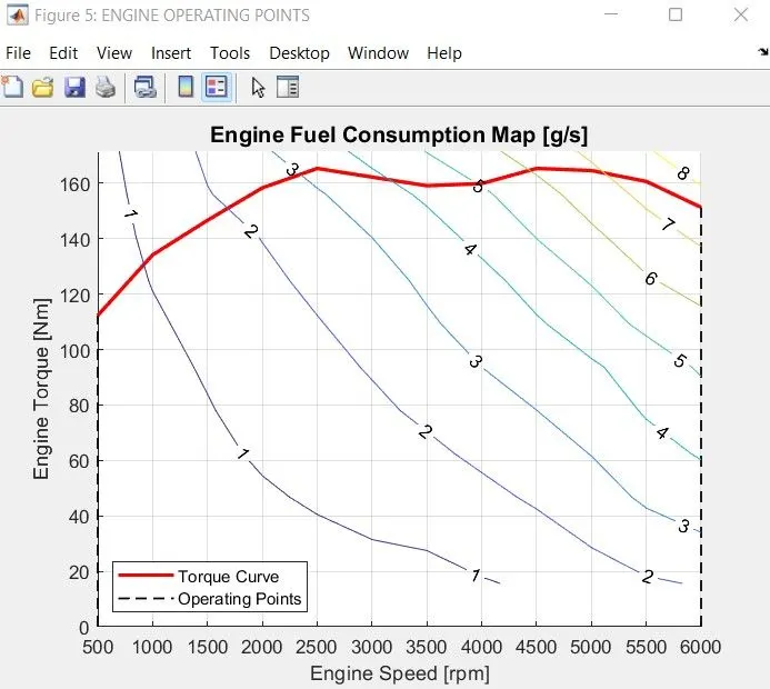
• The potting has been done for the maps with engine speed on x-axis and engine brake torque on y-axis, and the Engine operating points are represented using contour function.
• From the plotting, the engine maximum and minum torque's are identified and also the operating conditions are determined.
• The Engine fuel consumption is estimated by using the fuel map, based on the engine speed and engine torque @ operating conditions the fuel consumption of the vehicle is obtained.

f. Plotting the Electric Motor speed, Torque and Motor input power:

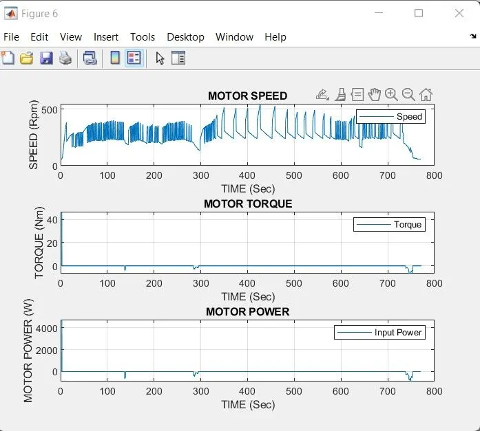
• The plot describes the Motor speed and Motor torque and motor power requirement.
• Based on the Electric motor torque and Electric motor speed the maximum and minimum torque are mapped using 1-D look up table and that are dynamically saturated using upper and lower limits from the Electric machine unit and by the electric motor control unit.
• The saturated executes the Electric power which are mapped using 2-D look up table from which the motor input power are mapped with respect to the electric motor speed and torque.
• The Electric power are used in determining the battery perfomance.

g.Plotting the Voltage, Current and State of charge using subplots:

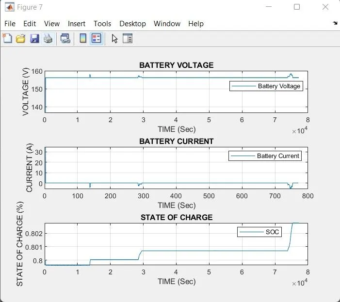
• Based on the time the Current (Amps), Voltage(V) and State of charge (SOC %) are varied accordingly.
• From the plotting it is obsorved that the initial state of charge would be 80% after the certain time intervel the state of charge will be varried according to the accelaration and delaration and regenerative braking commands by the control units as the discharging state..
• After that with constant time the SOC remains same as in the current are in constant state.
• Also. by considering the initial state of charge as 80% (0.8), to subtract with the determined SOC and saturated by using saturation block.
• The upper and lower limits are assigned as 0 and 1 of SOC during monetering and regenrative brakings.
• During charging, discharging and constant states the signals are varied respectively with same battery capacity as it connected in series.

h. Plotting the electric motor operating points on the motor input power map:

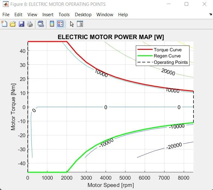
• The potting has been done for the maps with motor speed on x-axis and motor torque on y-axis, and the Electric motor points are represented using contour function.
• From the plotting, the motor monetering and generating torque's are identified and also the operating conditions are determined.
• The Regenerative braking is estimated by using the motor power map, based on the motor speed and motor torque @ operating conditions the power requirements of the vehicle is obtained.

ATTACHMENTS:

M-CODE- INITI-FILE:-

https://drive.google.com/file/d/1hjzLi_1zo9Q4iseAW6uWqfPsCb8Kqzci/view?usp=sharing

M- CODE POST PROCESSING FILE:-

https://drive.google.com/file/d/1FxhdlTkgrM7DY6gUvb6eN2TD3uR6oN70/view?usp=sharing

SIMULINK ATTACHMENT FILE:-

https://drive.google.com/drive/folders/1Xy6J4pym7ke6E_VYXmbvcKp9wtKqwkE0?usp=sharing

RESULT:

• From the UDDS and HWFET drive cycle's the fuel economy is obsorved as,
• In UDDS Drive cycle - 15.385
• In HWFET Drive cycle - 16.536
• Based on the fuel economy the HWFET drive cycle's has higher econnomy than UDDS drive cycle's, due to low braking and higher desired velocities.
• As, Compared to Conventioanl Internal combustion Engine, the P1 hybrid vehicle has higher fuel economy numbers in both UDDS and HWFET drive cycle's.

CONCLUSION:

• The development of a forward energy-based fuel consumption model of a P1 Hybrid vehicle by using simulink modells are created and analysed.
• The simulation on different drive cycles like UDDS, HWFET, FTP, NEDC,US06,WLDP using matlab scripts are done.
• The computation for the fuel economy numbers for the given vehicle (kmpl) on the urban cycle (UDDS) and highway cycle (HWFET) are carried out.
• The vehicle operating points in terms of engine speed, torque, transmission speeds, pedal positions, gear, distance travelled are analyzed.
• The time trace for engine, transmission input, transmission output and wheel speed on one plot are plotted.
• The engine torque, engine power, fuel rate and fuel consumption using subplots are plotted.
• The accelerator and brake pedal, gear command, vehicle desired and actual speed, vehicle distance using subplots are plotted.
• The engine operating points on the engine fuel map are carried out using contour function.
• The motor speed, torque, motor input power using subplots are carried out and analyzed.
• The battery pack voltage, current and SoC using subplots are plotted.
• The motor operating points on the motor input power map, with the motor max motoring and generating torque curves are plotted.
• The vehicle behavior throughout the drive cycle and the plots for both UDDS and HEFET cycle's are carried out.